Using Python in R Studio with Reticulate
By Sarah Murphy
Download all code used below from the GitHub repository!
There are four ways to use Python code in your R workflow:
- Python code blocks in R Markdown
- Interactively in the console
- Importing Python packages and using the commands within your R scripts
- Importing Python scripts and using user-defined functions within your R scripts
All of these require reticulate.
Reticulate
Reticulate is a library that allows you to open a Python environment within R. You can also load Python packages and use them within your R script using a mix of Python and R syntax. All data types will be converted to their equivalent type when being handed off between Python and R.
Installation
First, install the reticulate package:
1install.packages("reticulate")
When you install reticulate you are also installing Miniconda, a lightweight package manager for Python. This will create a new Python environment on your machine called r-reticulate. You do not need to use this environment but I will be using it for the rest of this post. More information about Python environments can be found here.
Python Code Blocks in R Markdown
R Markdown can contain both Python and R code blocks. When in an RMarkdown document you can either manually create a code block or click on the insert dropdown list in R Studio and select Python. Once you have a code block you can code using typical Python syntax. Python code blocks will run as Python code when you knit your document.

1## 6
Working with Python Interactively
We can use Python interactively within the console in R studio. To do this, we will use the repl_python() command. This opens a Python prompt.
 1# Load library
 2library(reticulate)
 3
 4# Open an interactive Python environment
 5# Type this in the console to open an interactive environment
 6repl_python()
 7
 8# We can do some simple Python commands
 9python_variable = 4
10print(python_variable)
11
12# To edit the interactive environment
13exit
You'll notice that when you're using Python >>> is displayed in the console. When you're using R, you should see >.
Changing Python environments
Using repl_python() will open the r-reticulate Python environment by default. If you've used Python and have a environment with packages loaded that you'd like to use, you can load that using the following commands.
1# I can see all my available Python versions and environments
2reticulate::py_config()
3
4# Load the Python installation you want to use
5use_python("/Users/smurphy/opt/anaconda3/envs/r-reticulate/bin/python")
6
7#  If you have a named environment you want to use you can load it by name
8use_virtualenv("r-reticulate")
Installing Python packages
Next, we need to install some Python packages:
1conda_install("r-reticulate", "cartopy", forge = TRUE)
2conda_install("r-reticulate", "matplotlib")
3conda_install("r-reticulate", "xarray")
The conda_install function uses Miniconda to install Python packages. We specify "r-reticulate" because that is the Python environment we want to install the packages into. We are going to install three different packages here, cartopy (for making maps), matplotlib (a common plotting package), and xarray (to import data).
Using Python Commands within R Scripts
We can now load our newly installed Python libraries in R. Open a new R script and import these packages using the import command. We are assigning these to some common nicknames for these packages so they are easier to reference later on.
1library(reticulate)
1## Warning: package 'reticulate' was built under R version 4.0.5
1plt <- import('matplotlib.pyplot')
2ccrs <- import('cartopy.crs')
3xr <- import('xarray')
4feature <- import('cartopy.feature')
Xarray comes with some tutorial datasets. We are going to use the air temperature tutorial dataset here. To import it, we will use the xarray open_dataset command. We can now use all the usual Python commands, substituting . for $.
1air_temperature <- xr$tutorial$open_dataset("air_temperature.nc")
2
3air_temperature
 1## <xarray.Dataset>
 2## Dimensions:  (lat: 25, lon: 53, time: 2920)
 3## Coordinates:
 4##   * lat      (lat) float32 75.0 72.5 70.0 67.5 65.0 ... 25.0 22.5 20.0 17.5 15.0
 5##   * lon      (lon) float32 200.0 202.5 205.0 207.5 ... 322.5 325.0 327.5 330.0
 6##   * time     (time) datetime64[ns] 2013-01-01 ... 2014-12-31T18:00:00
 7## Data variables:
 8##     air      (time, lat, lon) float32 ...
 9## Attributes:
10##     Conventions:  COARDS
11##     title:        4x daily NMC reanalysis (1948)
12##     description:  Data is from NMC initialized reanalysis\n(4x/day).  These a...
13##     platform:     Model
14##     references:   http://www.esrl.noaa.gov/psd/data/gridded/data.ncep.reanaly...
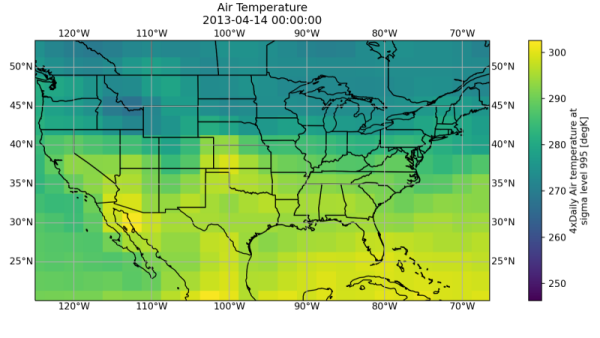
Next, we will create our figure. This is a map of air temperature over the United States for any day in 2013 specified in the plotting command.
Python users define lists with square brackets. However, the equivalent R type to this is a multi-element vector, so we must define it as such. One example of where this is used is in the first line in the following code block. In Python, we would specify the size of a figure using fig = plt.figure(figsize = [15, 5]), but when we use this command in R with reticulate we must use types that R recognizes, so we replace the = with <-, . with $, and [] with c() giving us fig <- plt$figure(figsize = c(15, 5)).
The Python equivalent of the following R code can be seen in the next section about sourcing Python scripts.
 1# Creating the figure
 2fig <- plt$figure(figsize = c(15, 5))
 3
 4# Defining the axes projection
 5ax <- plt$axes(projection = ccrs$PlateCarree())
 6
 7# Setting the latitude and longitude boundaries
 8ax$set_extent(c(-125, -66.5, 20, 50))
 9
10# Adding coastlines
11ax$coastlines()
12
13# Adding state boundaries
14ax$add_feature(feature$STATES);
15
16# Drawing the latitude and longitude
17ax$gridlines(draw_labels = TRUE);
18
19# Plotting air temperature
20plot <- air_temperature$air$sel(time='2013-04-14 00:00:00', method = 'nearest')$plot(ax = ax, transform = ccrs$PlateCarree())
21
22# Giving our figure a title
23ax$set_title('Air Temperature, 14 April 2013');
24
25plt$show()
1## <cartopy.mpl.feature_artist.FeatureArtist object at 0x00000000316F55F8>
1## <cartopy.mpl.gridliner.Gridliner object at 0x00000000316F5588>
1## Text(0.5, 1.0, 'Air Temperature\n2013-04-14 00:00:00')
1## <cartopy.mpl.feature_artist.FeatureArtist object at 0x0000000031726F28>
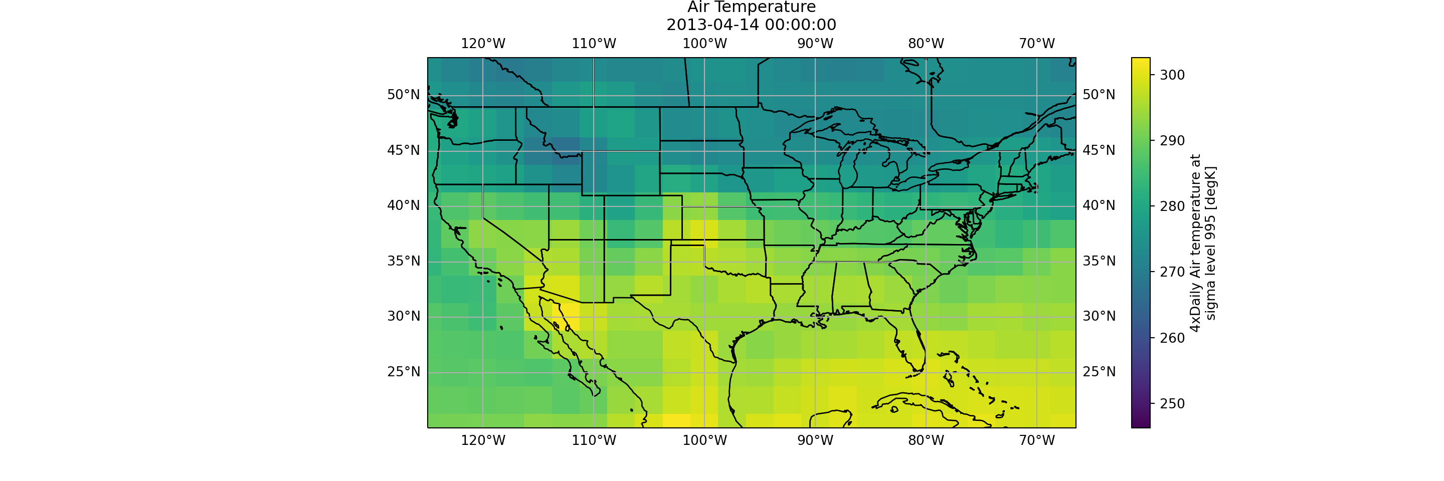
Sourcing Python Scripts
We can easily import a Python script and use user-defined functions from it using source_python. The Python script below creates a function that does the same thing as the above R script. This function accepts a date string and plots the corresponding map.
 1import xarray as xr
 2import matplotlib.pyplot as plt
 3import cartopy
 4import cartopy.crs as ccrs
 5
 6
 7def PlotAirTemp(usertime):
 8    """ Plot air temperature
 9    Args:
10        username (str): "yyyy-mm-dd hh:mm:ss"
11                (for example '2013-04-14 00:00:00')
12    """
13    air_temperature = xr.tutorial.open_dataset("air_temperature.nc")
14    fig = plt.figure(figsize = (15,5))
15    ax = plt.axes(projection = ccrs.PlateCarree())
16    ax.set_extent([-125, -66.5, 20, 50])
17    ax.coastlines()
18    ax.gridlines(draw_labels=True)
19    plot = air_temperature.air.sel(time=usertime).plot(ax = ax, transform = ccrs.PlateCarree())
20    ax.set_title('Air Temperature\n' + usertime)
21    ax.add_feature(cartopy.feature.STATES)
22    plt.show()
I have named the above file Python_PlotAirTemp.py. Once we source this file, we can use the function. Our function is called PlotAirTemp.
1library(reticulate)
2
3# Source the Python file to import the functions
4source_python('../Python_PlotAirTemp.py')
5
6# Call the function and give it the appropriate arguments
7PlotAirTemp('2013-04-14 00:00:00')
1## <cartopy.mpl.feature_artist.FeatureArtist object at 0x0000000032882E10>
1## <cartopy.mpl.gridliner.Gridliner object at 0x0000000032882DA0>
1## Text(0.5, 1.0, 'Air Temperature\n2013-04-14 00:00:00')
1## <cartopy.mpl.feature_artist.FeatureArtist object at 0x000000003287BB38>