Advanced methods with ggplot2

Sep 25, 2019 · 11 min read · cowplot ggplot2 ggpubr ggrepel tidyverse ·

This walkthrough will cover some advanced ways of working with ggplot2. There are a lot of functions and plotting options available in ggplot2, but here I'll be showing a couple of examples of ways to extend your ggplot2 usage with additional packages. This post is less about mind-blowing images as it is useful ways to produce and modify figures for your research.

Overview

This post is going to cover a couple of main points for working with ggplot2. They include:

Changing up color themes with viridis and labeling points with ggrepel
Generating multiple plots without copying and pasting code
Arranging multiple plots into one figure with a shared legend using ggpubr
Creating insets in a plot

Quick notes:

I'll be using pipes (%>%) in this post. You can find more info on their usage here if you haven't encountered them before
I assume you have some prior ggplot2 experience! Alli Cramer's Introduction to R post discusses some basic ggplot2 commands if you need them

The walkthrough

First off, we'll load the following packages:

1library(tidyverse)
2library(ggpubr)
3library(ggrepel)
4library(lubridate)
5library(tigris)
6library(sf)
7library(cowplot)

Next, we'll load in data exported from the iNaturalist website. The data are observations of animals, plants, fungi, and other forms of life from Whitman County, WA. You can download the file here.

1whitman_nature <- read.csv(file = "whitman_inaturalist.csv",
2                           stringsAsFactors = FALSE)

Most of the variables in this dataset are related to the taxonomic IDs of its observations.

1str(whitman_nature)

 1## 'data.frame':	3306 obs. of  32 variables:
 2##  $ observed_on           : chr  "2012-06-07" "2012-08-13" "2012-08-13" "2007-08-31" ...
 3##  $ quality_grade         : chr  "research" "research" "research" "research" ...
 4##  $ latitude              : num  46.7 46.7 46.7 47 46.7 ...
 5##  $ longitude             : num  -117 -117 -117 -117 -117 ...
 6##  $ coordinates_obscured  : chr  "false" "false" "false" "false" ...
 7##  $ species_guess         : chr  "Black-billed Magpie" "Gray Hairstreak" "Great Mullein" "Rock Wren" ...
 8##  $ scientific_name       : chr  "Pica hudsonia" "Strymon melinus" "Verbascum thapsus" "Salpinctes obsoletus" ...
 9##  $ common_name           : chr  "Black-billed Magpie" "Gray Hairstreak" "great mullein" "Rock Wren" ...
10##  $ iconic_taxon_name     : chr  "Aves" "Insecta" "Plantae" "Aves" ...
11##  $ taxon_id              : int  143853 50931 59029 7486 143853 9744 14823 2969 1409 13858 ...
12##  $ taxon_kingdom_name    : chr  "Animalia" "Animalia" "Plantae" "Animalia" ...
13##  $ taxon_phylum_name     : chr  "Chordata" "Arthropoda" "Tracheophyta" "Chordata" ...
14##  $ taxon_subphylum_name  : chr  "Vertebrata" "Hexapoda" "Angiospermae" "Vertebrata" ...
15##  $ taxon_superclass_name : chr  "" "" "" "" ...
16##  $ taxon_class_name      : chr  "Aves" "Insecta" "Magnoliopsida" "Aves" ...
17##  $ taxon_subclass_name   : chr  "" "Pterygota" "" "" ...
18##  $ taxon_superorder_name : chr  "" "" "" "" ...
19##  $ taxon_order_name      : chr  "Passeriformes" "Lepidoptera" "Lamiales" "Passeriformes" ...
20##  $ taxon_suborder_name   : chr  "" "" "" "" ...
21##  $ taxon_superfamily_name: chr  "" "Papilionoidea" "" "" ...
22##  $ taxon_family_name     : chr  "Corvidae" "Lycaenidae" "Scrophulariaceae" "Troglodytidae" ...
23##  $ taxon_subfamily_name  : chr  "" "Theclinae" "" "" ...
24##  $ taxon_supertribe_name : chr  "" "" "" "" ...
25##  $ taxon_tribe_name      : chr  "" "Eumaeini" "" "" ...
26##  $ taxon_subtribe_name   : chr  "" "Eumaeina" "" "" ...
27##  $ taxon_genus_name      : chr  "Pica" "Strymon" "Verbascum" "Salpinctes" ...
28##  $ taxon_genushybrid_name: logi  NA NA NA NA NA NA ...
29##  $ taxon_species_name    : chr  "Pica hudsonia" "Strymon melinus" "Verbascum thapsus" "Salpinctes obsoletus" ...
30##  $ taxon_hybrid_name     : chr  "" "" "" "" ...
31##  $ taxon_subspecies_name : chr  "" "" "" "" ...
32##  $ taxon_variety_name    : chr  "" "" "" "" ...
33##  $ taxon_form_name       : chr  "" "" "" "" ...

1. Some tweaks to a basic plot

Let's explore the dataset. For example, we might be interested in getting a sense of how common each group of organisms (plants, insects, mammals, etc.) is throughout the year. But before plotting we should prep the dataset a bit:

 1whitman_interest <- whitman_nature %>%
 2  # Remove missing dates
 3  filter(observed_on != "",
 4         # Focus on just groups with a lot of observations
 5         iconic_taxon_name %in% c("Insecta", "Plantae", "Mammalia",
 6                                  "Fungi", "Reptilia", "Amphibia")) %>%
 7  # Extract month and year data from the observed_on date
 8  mutate(month_obs = month(observed_on, label = TRUE),
 9         year_obs = year(observed_on)) %>%
10  # Count the number of observations by year, month, and taxonomic group
11  count(year_obs, month_obs, iconic_taxon_name) %>%
12  # Divide up the data by deciles so we can pick out times with peak sighting counts
13  mutate(n_tile = ntile(x = n, n = 10),
14         # Create a label denoting the data in the top decile of values
15         label = if_else(condition = n_tile == 10,
16                         true = as.character(year_obs), false = ""))
17
18head(whitman_interest)

1##   year_obs month_obs iconic_taxon_name  n n_tile label
2## 1     1993       Jun           Plantae 10      8      
3## 2     1993       Jul           Plantae  1      1      
4## 3     1997       Jun           Plantae  1      1      
5## 4     1998       Mar          Mammalia  1      1      
6## 5     2006       Jun           Plantae  1      1      
7## 6     2006       Sep          Mammalia  1      1

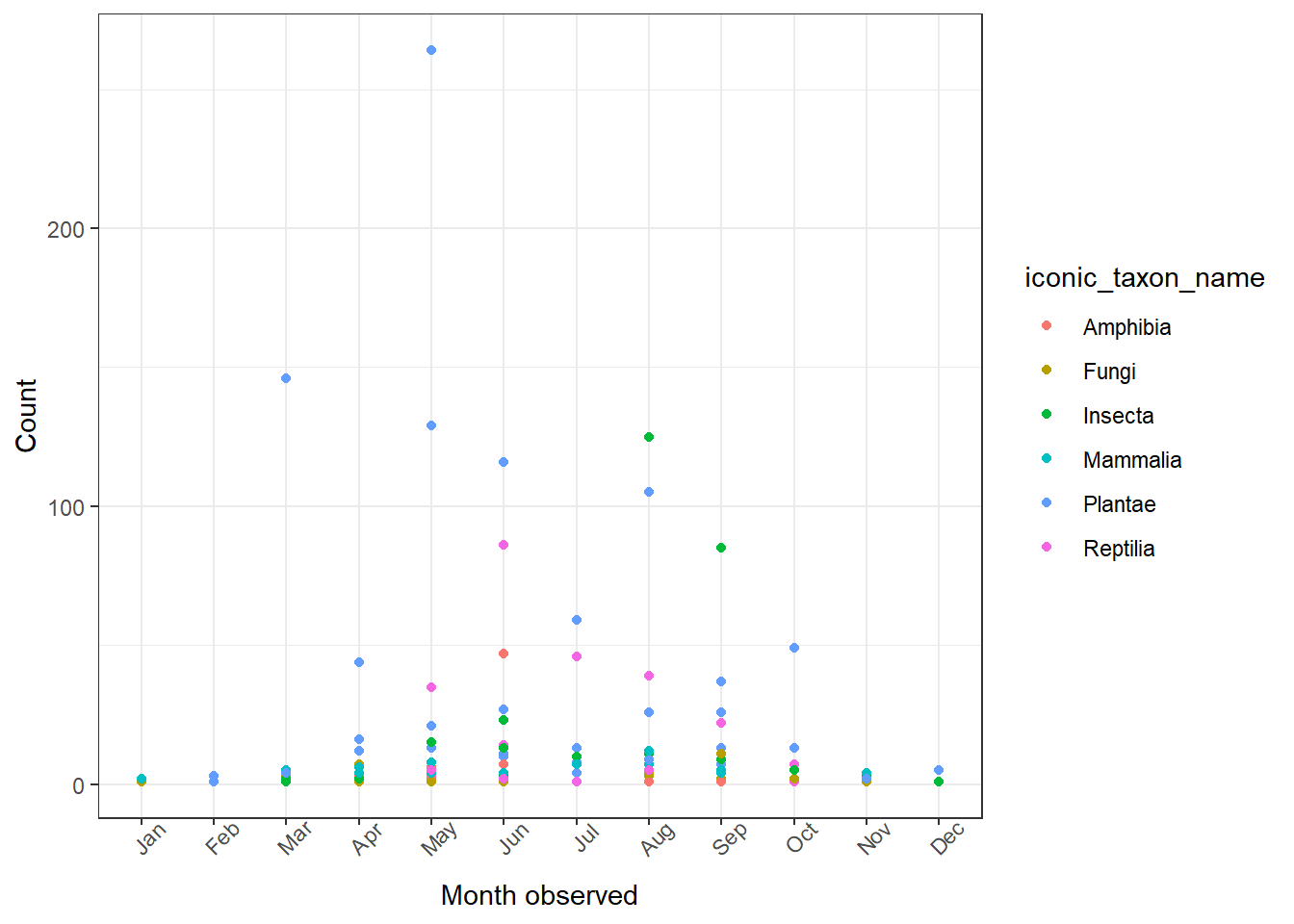
Now we'll plot what we've created above. Here's a basic start:

1ggplot(data = whitman_interest, aes(x = month_obs, y = n)) +
2  geom_point(aes(color = iconic_taxon_name)) +
3  theme_bw() +
4  theme(axis.text.x = element_text(angle = 45)) +
5  ylab(label = "Count") +
6  xlab(label = "Month observed")

This plot is fine, but there's more we can do with it. I've made a few changes below:

We use geom_text_repel() from ggrepel to place labels that don't overlap one another
We use scale_color_viridis_d() from ggplot2 to use a colorblind-friendly color palette
geom_jitter() adds some random variation to the point placement so that we don't have points overlapping one another

The viridis scale provides a colorblind-friendly palette to the color aesthetic we're using. Use scale_color_viridis_d() for discrete variables and scale_color_viridis_c() for continuous.

1ggplot(data = whitman_interest, aes(x = month_obs, y = n)) +
2  geom_jitter(aes(color = iconic_taxon_name)) +
3  geom_text_repel(aes(label = label)) +
4  scale_color_viridis_d(name = "Taxon name") +
5  theme_bw() +
6  theme(axis.text.x = element_text(angle = 45)) +
7  ylab(label = "Count") +
8  xlab(label = "Month observed")

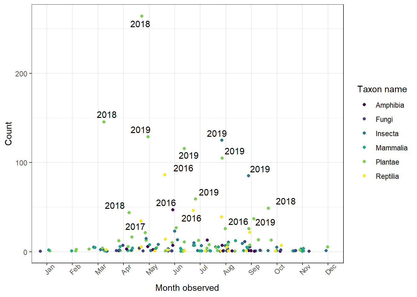
This plot now shows the counts of each taxonomic group during every month of the year in Whitman County. We can see that people generally report more observations during the middle of the year, but also more recent years have higher counts than earlier years (based on the labels). A label is placed for the month-species combinations that have counts in the highest 10%.

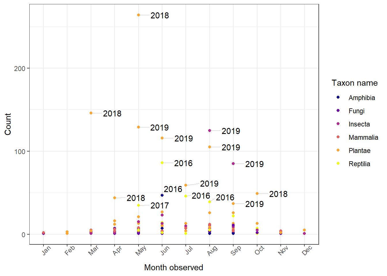
Note that if we want, we can change the viridis color palette and add line segments to the labels from ggrepel. As an example, we can change the color palette to "plasma" and add thin grey line segments. Here I also change geom_jitter() to geom_point() because the jitter doesn't line up with the geom_text_repel() segments well.

 1ggplot(data = whitman_interest, aes(x = month_obs, y = n)) +
 2  geom_point(aes(color = iconic_taxon_name)) +
 3  geom_text_repel(aes(label = label),
 4                  segment.size = 0.2, # Line width
 5                  min.segment.length = 0, # All labels have lines
 6                  nudge_x = 0.9, # Nudge x starting point of labels
 7                  segment.color = "gray") + # Line color
 8  scale_color_viridis_d(name = "Taxon name", option = "plasma") +
 9  theme_bw() +
10  theme(axis.text.x = element_text(angle = 45)) +
11  ylab(label = "Count") +
12  xlab(label = "Month observed")

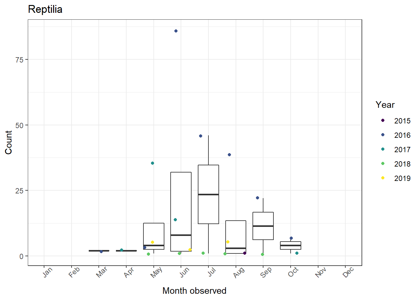
2. What if we wanted to generate a plot for each group?

The plot above is generally informative, but what if you wanted to break it out so that you had a separate plot for each taxonomic group (i.e., insects, plants, etc.)?

It might look like this:

 1ggplot(data = whitman_interest %>%
 2         filter(iconic_taxon_name == "Plantae"),
 3       aes(x = month_obs, y = n)) +
 4  geom_boxplot(outlier.shape = NA) +
 5  geom_jitter(aes(color = factor(year_obs))) +
 6  scale_color_viridis_d(name = "Year") +
 7  theme_bw() +
 8  theme(axis.text.x = element_text(angle = 45)) +
 9  ggtitle(label = "Plantae") +
10  ylab(label = "Count") +
11  xlab(label = "Month observed")

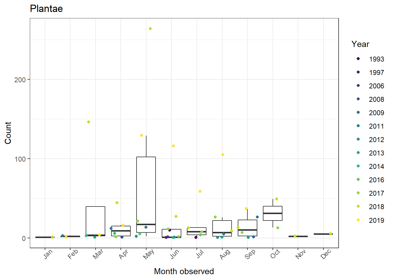
This gives us a plants plot, but none of the taxonomic other groups. If you're like me, you've got a few scripts lying around where you just copied and pasted the same code a bunch of times to make multiple figures. Luckily there's a simpler, more reliable way for us to produce plots for each taxonomic group in this case.

Recall that we have the column iconic_taxon_name with the values Plantae, Mammalia, Insecta, Fungi, Reptilia, Amphibia.

Using the function map() from the package purrr, we can produce a new plot for each value in a vector that we specify. In this case, we'll supply a vector of the unique values of iconic_taxon_name and tell R to use each value (e.g. "Plantae") to filter the dataset and create a plot title:

The basic structure of `purrr::map()`:

1map(.x = , # Here we supply the vector of values (in this case taxa names)
2    .f = ~ ) # Here we supply the function we want to feed those values into

We'll want to provide a function that can use any of the inputs in our taxa vector. Instead of writing the taxa name (e.g. "Plantae") in our function, we'll replace it with .x, which is the name of the first argument in the map() function:

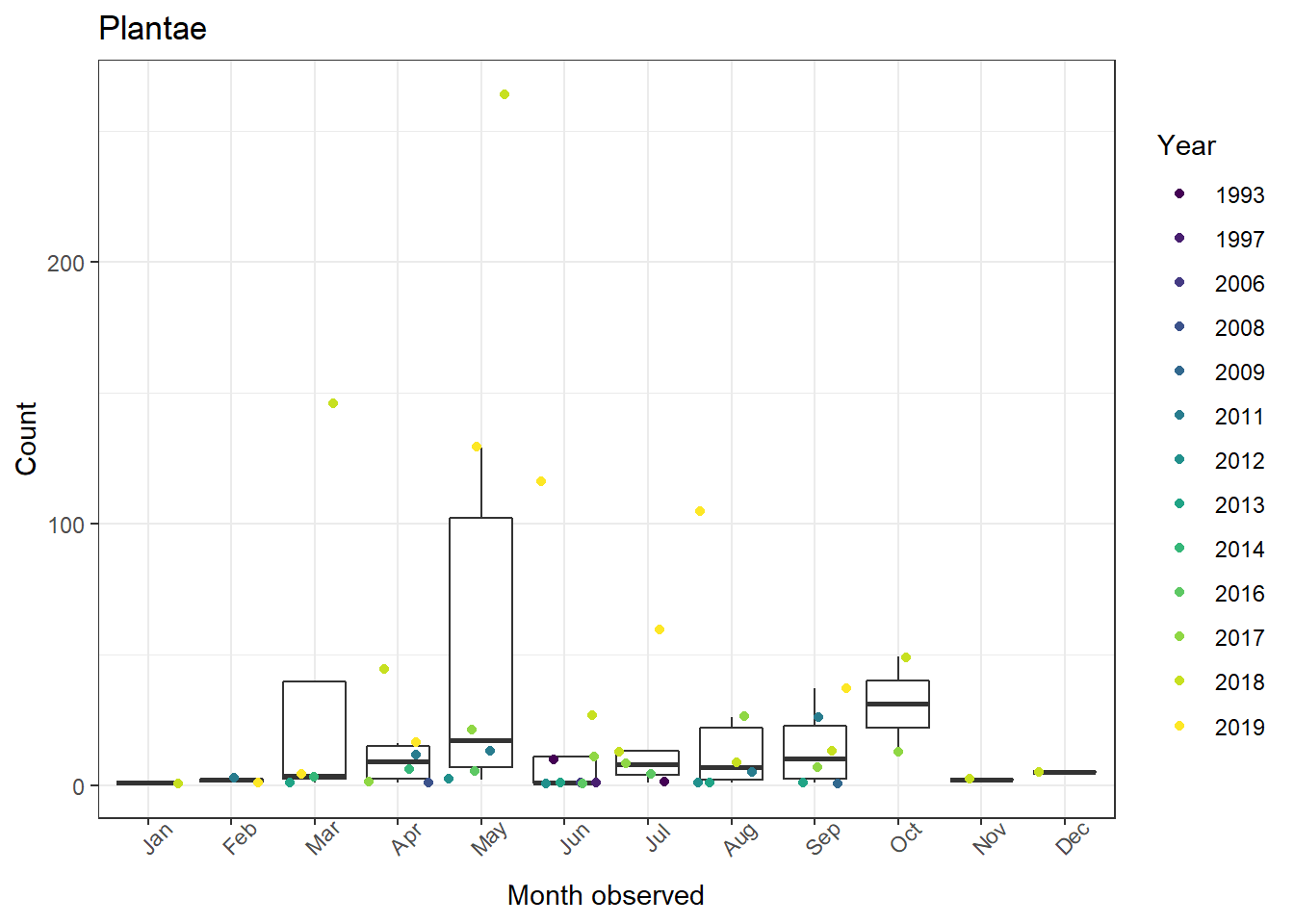
 1whitman_interest %>%
 2              filter(iconic_taxon_name == .x) %>%
 3              ggplot(aes(x = month_obs, y = n)) +
 4              geom_boxplot(outlier.shape = NA) +
 5              geom_jitter(aes(color = factor(year_obs))) +
 6              scale_color_viridis_d(name = "Year") +
 7              scale_x_discrete(drop = FALSE) + # Include months with no data
 8              theme_bw() +
 9              theme(axis.text.x = element_text(angle = 45)) +
10              ggtitle(label = .x) +
11              ylab(label = "Count") +
12              xlab(label = "Month observed")

Now if we combine our vector of taxa names and this function, we get a full map() call. Note the use of the ~ before the function call:

 1figs <- map(.x = c(unique(whitman_interest$iconic_taxon_name)),
 2            .f = ~ whitman_interest %>%
 3              filter(iconic_taxon_name == .x) %>%
 4              ggplot(aes(x = month_obs, y = n)) +
 5              geom_boxplot(outlier.shape = NA) +
 6              geom_jitter(aes(color = factor(year_obs))) +
 7              scale_color_viridis_d(name = "Year", drop = FALSE) +
 8              scale_x_discrete(drop = FALSE) +
 9              theme_bw() +
10              theme(axis.text.x = element_text(angle = 45)) +
11              ggtitle(label = .x) +
12              ylab(label = "Count") +
13              xlab(label = "Month observed"))

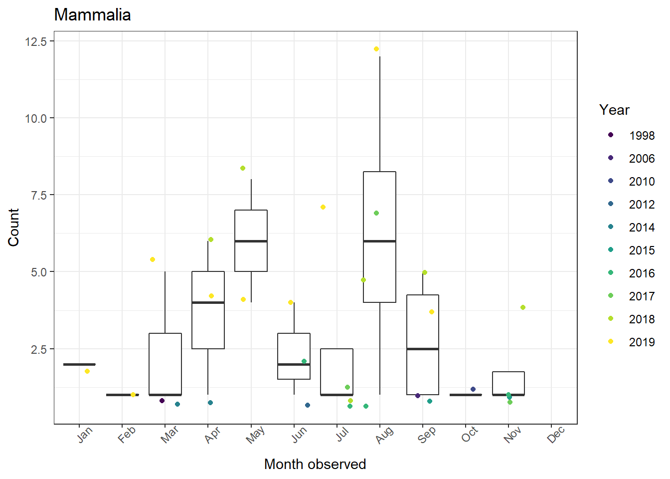
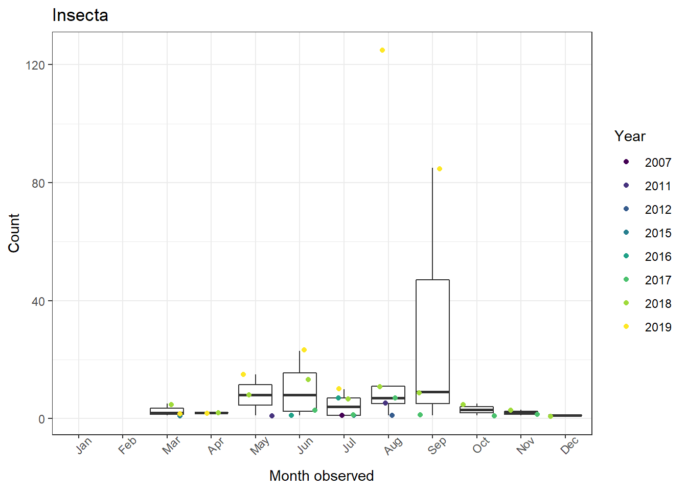
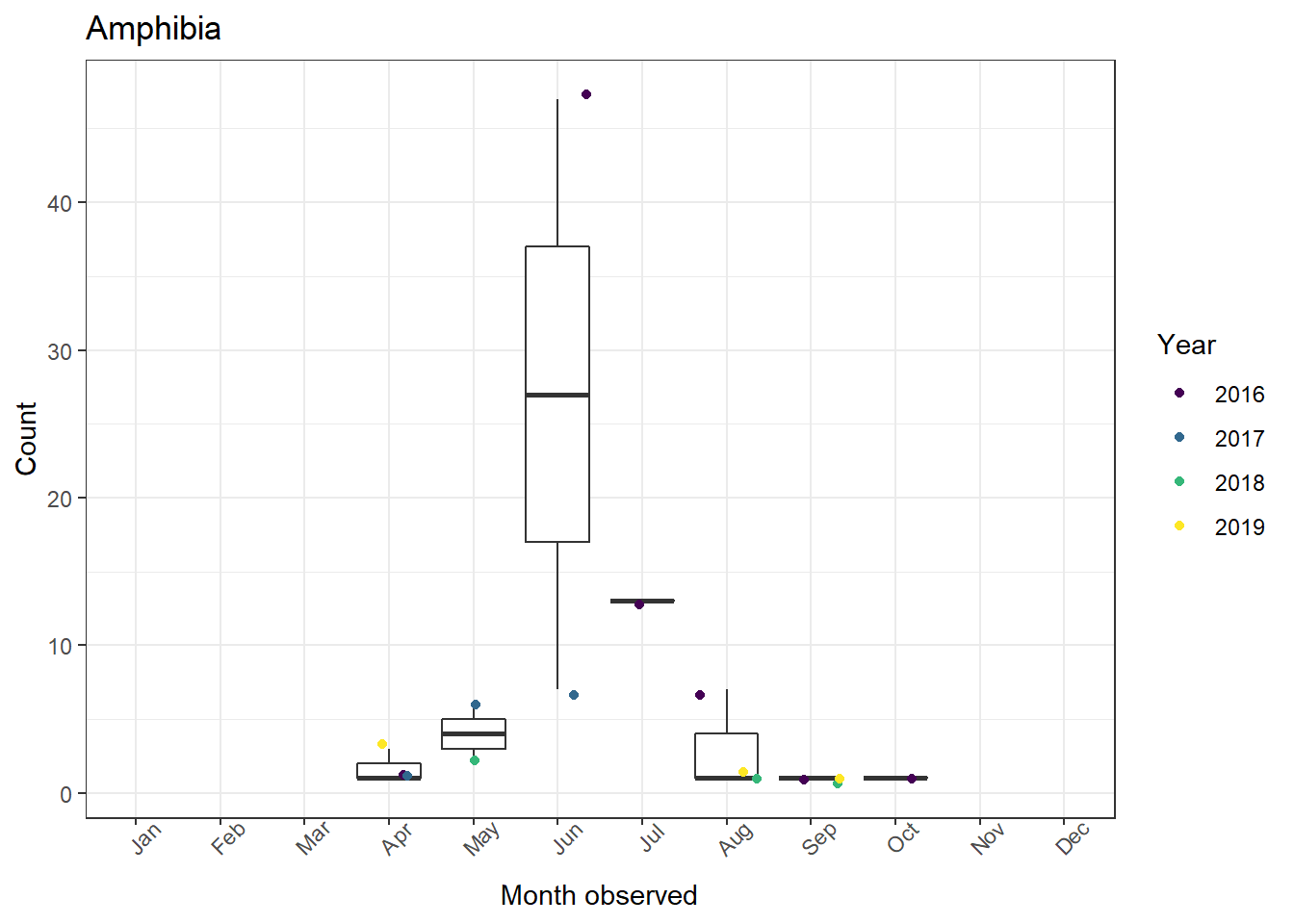
The figs object is now a list of figures for all six of our taxa!

1typeof(figs)

1## [1] "list"

1figs

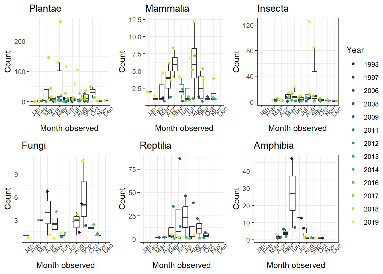
3. Combining figures into one plot

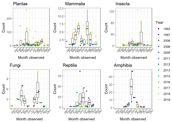
Now that we have all six figures we want, we might want to combine them into a single plot. This is possible using ggarrange() from ggpubr. We just need to supply it our plot list (figs). We can even have it use create one legend for all six plots!

1ggarrange(plotlist = figs, # List of our plots to arrange
2          common.legend = TRUE, # One legend for all plots (only if it makes sense!)
3          legend = "right") # Place legend on right side of figure

There are ways that you can use this method to have single x- or y-axis labels, too, but I won't cover that here in detail. Essentially, you leave the axis titles of the individual plots blank and then use the ggpubr annotate_figure() function to create new axis labels for the entire figure.

4. Insets

Mapping in ggplot2 deserves its own separate treatment so I won't cover the backround right now, but creating maps provides great context for plot insets. A plot inset is a smaller plot or image included within a larger one. For example, you may want to include a zoomed out map for spatial context alongside your regular map.

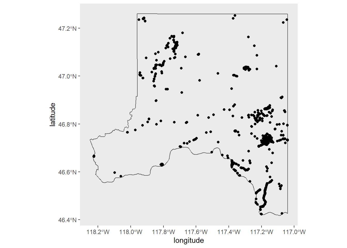
We can continue using the iNaturalist data and ggplot2 for this. Let's plot the locations where people have made observations.

First get the Whitman county shapefile. st_as_sf() comes from the sf package, while counties() comes from tigris.

1whitman_co <- st_as_sf(counties(state = "Washington", cb = TRUE)) %>% filter(NAME == "Whitman")

Then make a basic map with observation points.

 1whitman_map_data <- whitman_nature %>% filter(coordinates_obscured == "false")
 2
 3whitman_point <- ggplot() +
 4  geom_sf(data = whitman_co, fill = NA) +
 5  geom_point(data = whitman_map_data,
 6             aes(x = longitude, y = latitude)) +
 7  scale_fill_viridis_c() +
 8  theme(panel.grid = element_blank())
 9
10whitman_point

We go about creating the inset map much like the regular one. I add a filled black polygon for Whitman County over the Washington polygon and simplified the style of the map compared with the larger focal map.

 1washington_st <- st_as_sf(states()) %>% filter(NAME == "Washington")
 2
 3inset_map <- ggplot() +
 4  geom_sf(data = washington_st,
 5          fill = NA) +
 6  geom_sf(data = whitman_co,
 7          fill = "black") +
 8  theme_bw() +
 9  xlab("") +
10  ylab("") +
11  theme(axis.title.x = element_blank(),
12        axis.title.y = element_blank(),
13        panel.grid = element_blank(),
14        axis.text = element_blank(),
15        axis.ticks = element_blank(),
16        plot.background = element_blank())

We can now place the inset using ggdraw() and draw_plot() from cowplot.

1ggdraw() +
2  draw_plot(whitman_point) +
3  draw_plot(plot = inset_map,
4            x = 0.085, # x location of inset placement
5            y = 0.04, # y location of inset placement
6            width = .455, # Inset width
7            height = .26, # Inset height
8            scale = .58) # Inset scale

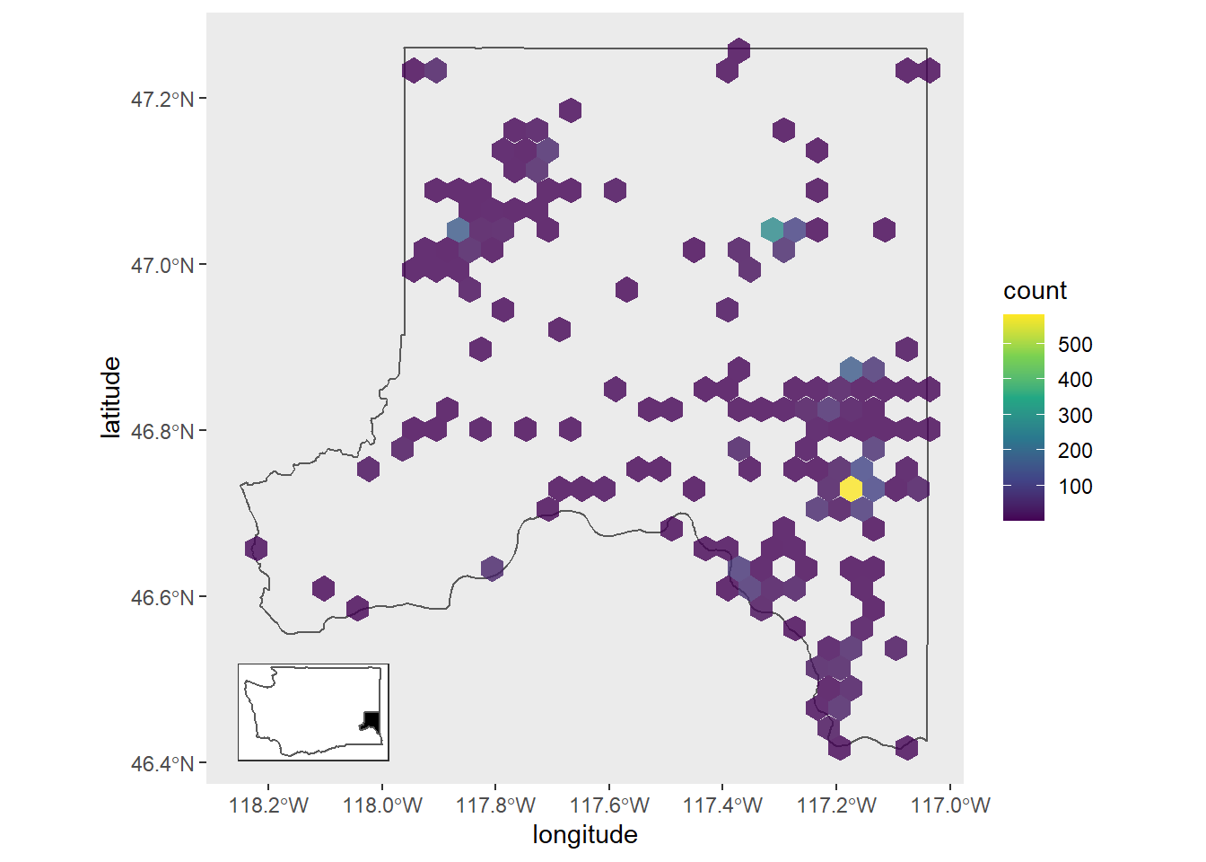
There's some overplotting of points on our map. One way we can deal with this and spice the map up a bit would be to replace the point layer with a heatmap hex layer (geom_hex()). Also, the plot inset moves if we use the same xy location as in the previous plot so I've changed the xy info.

 1whitman_hex <- ggplot() +
 2  geom_sf(data = whitman_co, fill = NA) +
 3  geom_hex(data = whitman_map_data,
 4           aes(x = longitude, y = latitude),
 5           alpha = 0.8) + # Partial transparency
 6  scale_fill_viridis_c() +
 7  theme(panel.grid = element_blank())
 8
 9ggdraw() +
10  draw_plot(whitman_hex) +
11  draw_plot(plot = inset_map,
12            x = 0.03,
13            y = 0.04,
14            width = .455,
15            height = .26,
16            scale = .58)

References

iNaturalist. Available from https://www.inaturalist.org. Accessed 2019-09-12.