A Tour of R Markdown
By Matt Brousil
Graduate students and other researchers often find themselves pasting figures or
tables into Microsoft Word or other word processing software in order to share
them with collaborators or PIs. Anyone who has tried to format text and images in
the same Word document knows that this is a harrowing experience. Luckily, the
rmarkdown package in R allows us to avoid this altogether.
R Markdown lets us combine narrative text
(e.g., an Intro, Methods, Discussion) with code (R or some other languages),
figures, and even interactive effects. Not only can this be more reliable than
using software like Word, it is also more reproducible and allows us to explain
the thoughts behind our scripts in the same file we use to flesh out the script.
R Markdown's capabilities are also very extensive. You can generate things like HTML, PDF, or Word reports; websites (like this blogs post!); slideshows; and interactive documents that use Shiny.
In this walkthrough we'll take a look at the basics of R Markdown and finish up by generating an example report. It will look something like this:
1. Install
The first thing you'll need to do is install some packages. The process is described by Yihui Xie here but if you are an RStudio user, the general process is:
- Install the
rmarkdownandtinytexpackages. - Use the function
tinytex::install_tinytex()to give yourself the ability to generate PDF documents via LaTex with R Markdown.
2. Basic overview
Before getting started, note that I am writing this walkthrough with RStudio users in mind. If you don't use RStudio, you should refer to Yihui Xie's instructions again.
To get started making an R Markdown document, you can go to File > New File > R Markdown in RStudio. This will generate a pop-up that looks like this:
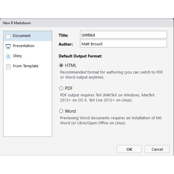
Provide it with a title for your document, the name of the author, and the type of document that you'd like to produce. HTML is typically the most reliable in my experience, and it often is best at formatting large tables and R console output.
Click OK and you should have a document that looks like this:
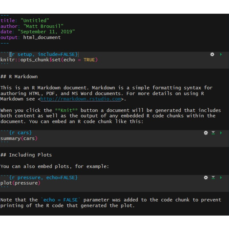
Note that there are three parts to this document.
The top of the document has a header that looks like this:
1---
2title: "Untitled"
3author: "Matt Brousil"
4date: "September 11, 2019"
5output: html_document
6---
This YAML text specifies some of the header info and formatting of your output document. There are guidelines on editing it here.
Then there is plain text in the main document:
This is how you include narrative text within your document. It will be rendered pretty much as you see it in the final document, but there are options to do things like bold the text, add links, images, etc.
Lastly, there are code chunks. These will be in the R language for us, but you
can include several other languages as well.
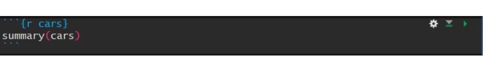
These chunks of code are run by R when you compile your final document. Each code chunk can be run using the green arrow on the right side of the chunk.
Feel free to just delete everything in your new R Markdown document except the YAML header for our example. Then go ahead and save. You'll notice that the filetype for the R Markdown document is .Rmd
How to create the output HTML or PDF files?
At any time you can have R generate the HTML or PDF file you're hoping to create
by clicking the Knit button.
 This also includes a dropdown that will let you
switch between PDF, HTML, and Word outputs.
This also includes a dropdown that will let you
switch between PDF, HTML, and Word outputs.
Basic syntax
There are a few key things you'll want to know how to do in R Markdown.
2.1. Make headers
In R Markdown you can make headers using the # symbol. There are several tiers:
# The biggest header
The biggest header
## The second biggest header
The second biggest header
###### The smallest header
The smallest header
2.2. Write basic text
To write normal text, just type within the main document as you normally would in a word processing program. For example:
The following section contains the results of my statistical analysis. After
performing this analysis I found a significant relationship between my variable of
interest and the experimental treatments.
The following section contains the results of my statistical analysis. After performing this analysis I found a significant relationship between my variable of interest and the experimental treatments.
However, do note that you'll need to include two spaces at the end of a line to create line breaks in your raw text. This is easily overlooked.
2.3. Format text
You can bold and italicize text using asterisks (*):
**bold text**
bold text
*italic text*
italic text
You can also do other things such as
super^script^
super^script^
and adding links:
[the text to display](www.google.com)
2.4. Add in code!
Here's the fun part! Now that we know how to insert and format text, you can also
add in chunks of R code. Go to Code > Insert Chunk in RStudio to insert a chunk.
You can also just type out a chunk manually using backticks and {r} to indicate
R language.
```{r}
print("My first R Markdown code")
```
R will show both the code and its result, by default.
1print("My first R Markdown code")
1## [1] "My first R Markdown code"
In some cases you might want to include code but not print it out in the final
document, e.g. including only the resulting figure or result. You can hide the
raw code using echo = FALSE:
```{r echo=FALSE}
print("My first R Markdown code")
```
1## [1] "My first R Markdown code"
Code can be inserted into your narrative text (e.g. in a sentence) by using backticks with the letter 'r':
The iris dataset contains the following column names: `r names(iris)`.
The iris dataset contains the following column names: Sepal.Length, Sepal.Width, Petal.Length, Petal.Width, Species.
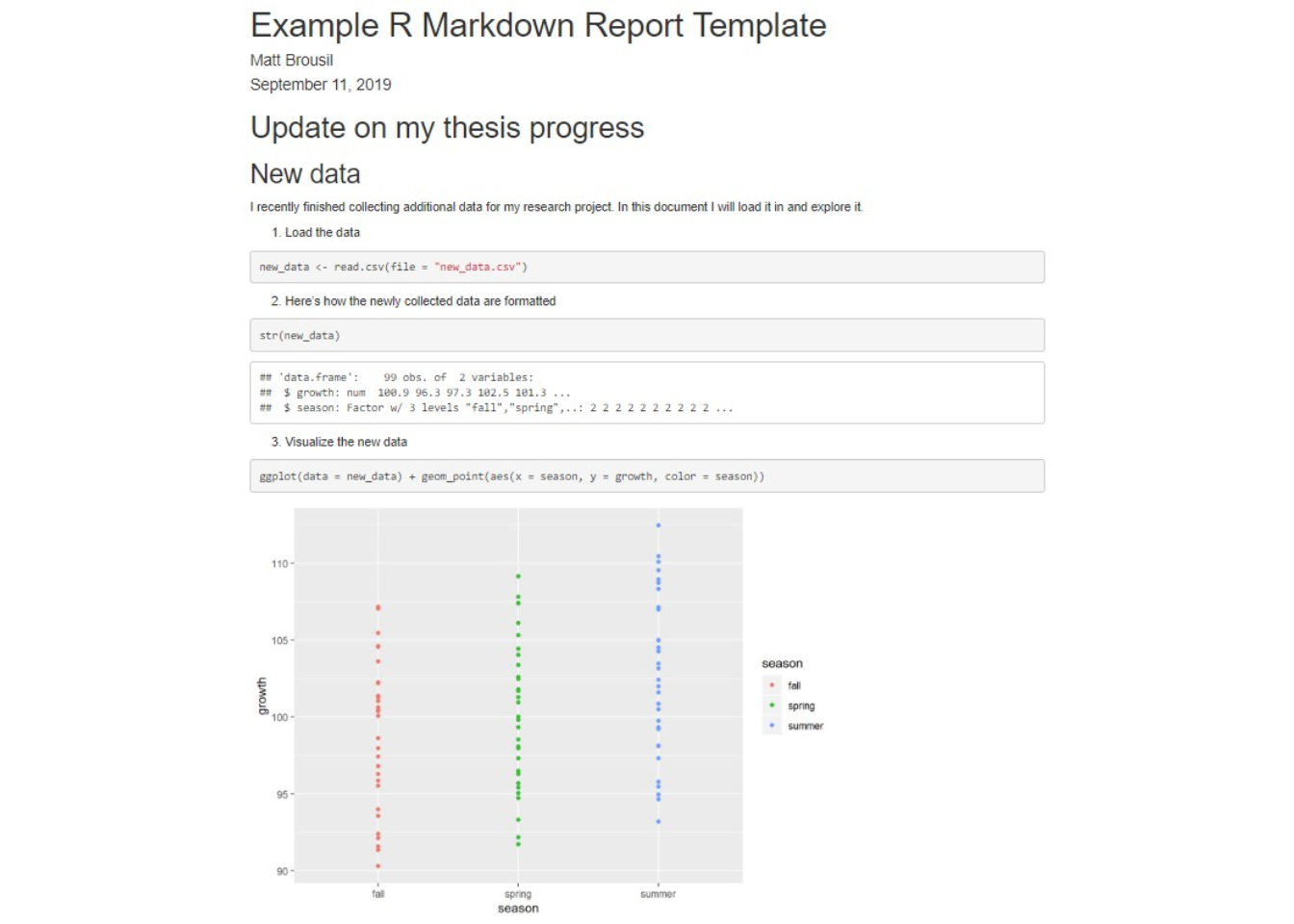
3. Report example
Now let's put the topics from the above section together! Below I provide a very brief template (and its knitted output) showing how you might write up a post-analysis report to share with an advisor or PI. There's plenty to customize, but this is a skeleton that might be of use. You can download this script as a .Rmd file here along with the associated dataset.
The script:
# Update on my thesis progress
```{r echo=FALSE, message=FALSE, warning=FALSE}
# This chunk won't be printed: We're just loading a package, so it might not be something that we want to have take up space in the final doc.
library(tidyverse)
library(ggpubr)
library(knitr)
```
## New data
I recently finished collecting additional data for my research project. In this
document I will load it in and explore it.
1. Load the data
```{r, }
new_data <- read.csv(file = "new_data.csv")
```
2. Here's how the newly collected data are formatted
```{r}
str(new_data)
sample_n(tbl = new_data, size = 20)
```
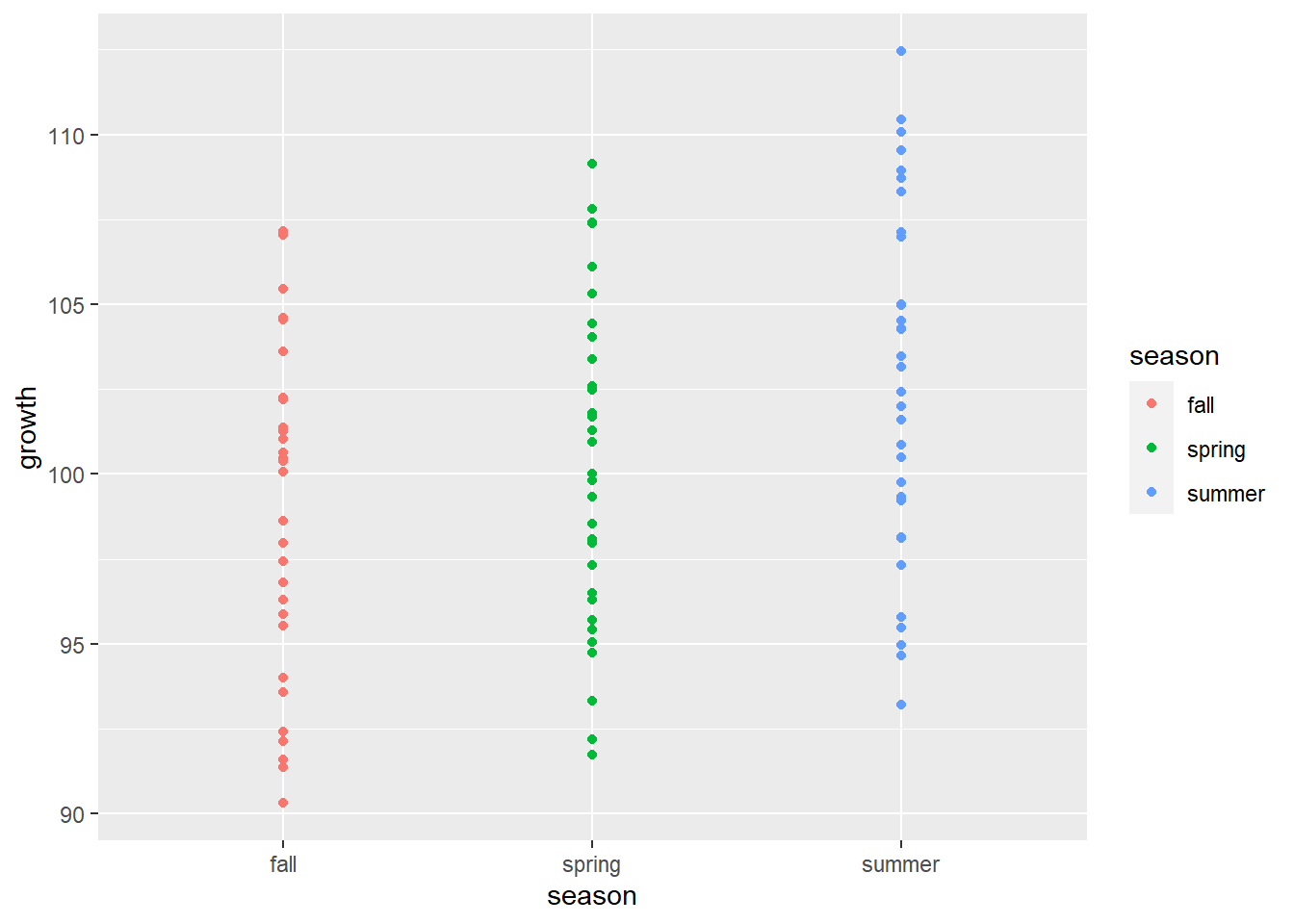
3. Visualize the new data
```{r}
ggplot(data = new_data) +
geom_point(aes(x = season, y = growth, color = season))
```
4. I ran a statistical test on the new data. Here are the results
```{r}
new_anova <- lm(formula = growth ~ season, data = new_data)
anova(new_anova) %>% kable()
```
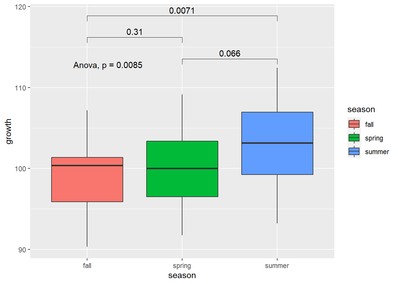
5. Now I plot the significance to illustrate the results
```{r}
ggplot(data = new_data,
aes(x = season, y = growth, fill = season)) +
geom_boxplot() +
stat_compare_means(comparisons = list(c("spring", "summer"),
c("spring", "fall"),
c("summer", "fall"))) +
stat_compare_means(method = "anova")
```
The knitted output:
Update on my thesis progress
New data
I recently finished collecting additional data for my research project. In this document I will load it in and explore it.
- Load the data
1new_data <- read.csv(file = "new_data.csv")
- Here's how the newly collected data are formatted
1str(new_data)
1## 'data.frame':	99 obs. of  2 variables:
2##  $ growth: num  100.9 96.3 97.3 102.5 101.3 ...
3##  $ season: chr  "spring" "spring" "spring" "spring" ...
1sample_n(tbl = new_data, size = 20)
 1##       growth season
 2## 1  103.16409 summer
 3## 2   91.36536   fall
 4## 3   97.43616   fall
 5## 4   91.59732   fall
 6## 5  103.16286 summer
 7## 6  102.25230   fall
 8## 7   99.32137 summer
 9## 8   96.80343   fall
10## 9  100.50303 summer
11## 10  97.32140 spring
12## 11 109.53290 summer
13## 12  94.64687 summer
14## 13 101.69457 spring
15## 14 100.36823   fall
16## 15 101.03978   fall
17## 16 100.43983   fall
18## 17  97.98659 spring
19## 18  99.34483 spring
20## 19 100.62673   fall
21## 20 108.72072 summer
- Visualize the new data
1ggplot(data = new_data) +
2  geom_point(aes(x = season, y = growth, color = season))
- I ran a statistical test on the new data. Here are the results
1new_anova <- lm(formula = growth ~ season, data = new_data)
2
3anova(new_anova) %>% kable()
| Df | Sum Sq | Mean Sq | F value | Pr(>F) | |
|---|---|---|---|---|---|
| season | 2 | 233.8816 | 116.94082 | 5.015241 | 0.008479 |
| Residuals | 96 | 2238.4406 | 23.31709 | NA | NA |
- Now I plot the significance to illustrate the results
1ggplot(data = new_data,
2       aes(x = season, y = growth, fill = season)) +
3  geom_boxplot() +
4  stat_compare_means(comparisons = list(c("spring", "summer"),
5                                        c("spring", "fall"),
6                                        c("summer", "fall"))) +
7  stat_compare_means(method = "anova")
4. References:
- https://bookdown.org/yihui/rmarkdown/
- https://bookdown.org/yihui/bookdown/r-markdown.html
- https://rmarkdown.rstudio.com/
- http://www.sthda.com/english/articles/24-ggpubr-publication-ready-plots/76-add-p-values-and-significance-levels-to-ggplots/
Cheat sheets:
Additionally, there are some great cheat sheets available for R Markdown: