An introduction to linear models with R
By Mikala Meize
Libraries used
1library(QuantPsyc)
2library(lmtest)
3library(palmerpenguins)
Linear model information
Linear models are generally coded in this format: model.name <- modeltype(outcome ~ predictor, data, specifications)
The following code will apply specifically to Ordinary Least Squares (OLS) regression; these use continuous outcome/dependent variables.
We will use the mtcars dataset that comes with R and the penguins dataset that comes with the 'palmerpenguins' library for these examples.
Linear models with one predictor
Outcome variable: mtcars$mpg
1#checking for normal distribution in the outcome variable
2hist(mtcars$mpg)

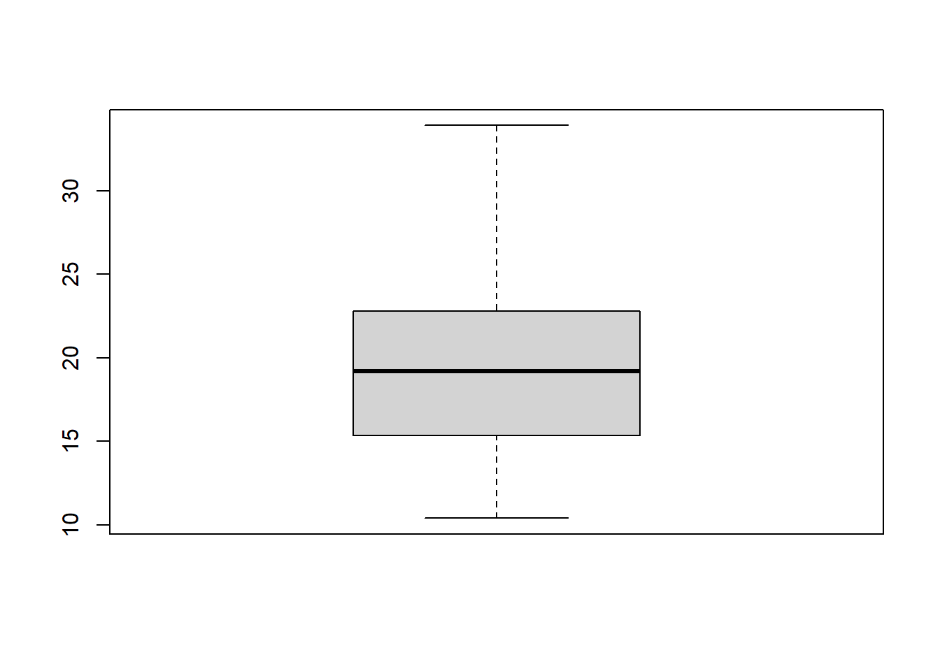
1#checking for outliers
2boxplot(mtcars$mpg)
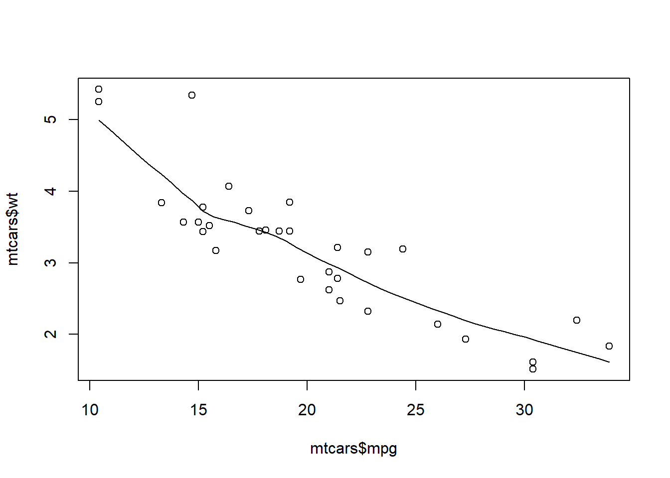
Predictor variable: mtcars$wt Checking for a linear relationship between outcome and predictor variables using a plot() code:
1plot(mtcars$mpg, mtcars$wt)

1scatter.smooth(mtcars$mpg, mtcars$wt)
Just for some useful information - checking the strength of that linear relationship using correlations codes. Both of these codes give us the correlation between the variables, but cor.test() outputs the results of a significance test.
 1cor(mtcars$mpg, mtcars$wt) #correlation between x and y variables
 2
 3## [1] -0.8676594
 4
 5cor.test(mtcars$mpg, mtcars$wt) #correlation with significance test
 6
 7##
 8##  Pearson's product-moment correlation
 9##
10## data:  mtcars$mpg and mtcars$wt
11## t = -9.559, df = 30, p-value = 1.294e-10
12## alternative hypothesis: true correlation is not equal to 0
13## 95 percent confidence interval:
14##  -0.9338264 -0.7440872
15## sample estimates:
16##        cor
17## -0.8676594
Code for single predictor linear model
The code for a linear model using a single predictor follows the basic format given above.
- Model type: lm()
- Outcome: mpg
- Predictor: Weight (wt)
- Data: mtcars
1mpg.model <- lm(mpg ~ wt, mtcars)
The model shows up in the global environment. To see the results of the model, run a summary() code.
 1summary(mpg.model)
 2
 3##
 4## Call:
 5## lm(formula = mpg ~ wt, data = mtcars)
 6##
 7## Residuals:
 8##     Min      1Q  Median      3Q     Max
 9## -4.5432 -2.3647 -0.1252  1.4096  6.8727
10##
11## Coefficients:
12##             Estimate Std. Error t value Pr(>|t|)
13## (Intercept)  37.2851     1.8776  19.858  < 2e-16 ***
14## wt           -5.3445     0.5591  -9.559 1.29e-10 ***
15## ---
16## Signif. codes:  0 '***' 0.001 '**' 0.01 '*' 0.05 '.' 0.1 ' ' 1
17##
18## Residual standard error: 3.046 on 30 degrees of freedom
19## Multiple R-squared:  0.7528, Adjusted R-squared:  0.7446
20## F-statistic: 91.38 on 1 and 30 DF,  p-value: 1.294e-10
Interpreting the results of a single predictor linear model
- The F-test/Anova at the end of the results is statistically significant. This means our model with one predictor is stronger than a null model with no predictors.
- The Multiple R-Squared value indicates that the predictor (weight) explains about 75% of the variance in the outcome (miles per gallon). The Adjusted R-Squared value has the same interpretation as the Multiple R-Squared value, but penalizes more complex models. As we increase predictors, the multiple R-squared is expected to increase simply because we added something else to explain the outcome; however, the adjusted R-squared value penalizes models because it's possible we've added a variable that does not actually increase the explanatory power of our model.
- The predictor (weight) is statistically significant and the coefficient is negative. This matches the visual relationship in the plot() code from above. Simply put, as the weight of a car increases, the miles per gallon decreases.
The format of an equation for a linear model is: Outcome = Intercept + Coefficient*Predictor If we put these values into an equation, it would look like this:
- mpg = 37.2851 - 5.3445(weight)
Linear models with two or more predictors
- Outcome variable: mtcars$mpg
- Predictor variable 1: mtcars$wt
- Predictor variable 2: mtcars$hp
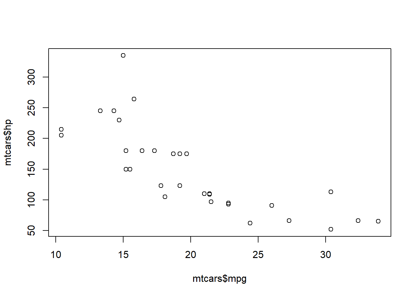
The relationship between mpg and wt has not changed in the data, so when we add a predictor, we only run the linear checks and such on the second predictor. Checking for a linear relationship between outcome and predictor variable 2 using a plot() code:
1plot(mtcars$mpg, mtcars$hp)
1scatter.smooth(mtcars$mpg, mtcars$hp)
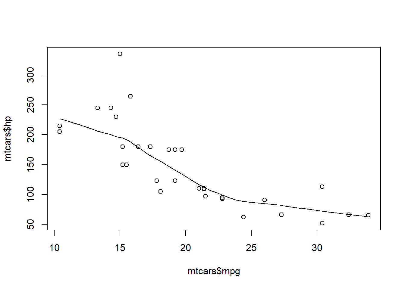
Just for some useful information - checking the strength of that linear relationship using correlations codes. Both of these codes give us the correlation between the variables, but cor.test() outputs the results of a significance test.
 1cor(mtcars$mpg, mtcars$hp) #correlation between x and y variables
 2
 3## [1] -0.7761684
 4
 5cor.test(mtcars$mpg, mtcars$hp) #correlation with significance test
 6
 7##
 8##  Pearson's product-moment correlation
 9##
10## data:  mtcars$mpg and mtcars$hp
11## t = -6.7424, df = 30, p-value = 1.788e-07
12## alternative hypothesis: true correlation is not equal to 0
13## 95 percent confidence interval:
14##  -0.8852686 -0.5860994
15## sample estimates:
16##        cor
17## -0.7761684
Code for multiple predictor linear model
The code for a linear model using a multiple predictor follows the basic format given above.
- Model type: lm()
- Outcome: mpg
- Predictor(s): weight (wt) + horsepower (hp)
- Data: mtcars
1mpg.model2 <- lm(mpg ~ wt + hp, mtcars)
The model shows up in the global environment. To see the results of the model, run a summary() code.
 1summary(mpg.model2)
 2
 3##
 4## Call:
 5## lm(formula = mpg ~ wt + hp, data = mtcars)
 6##
 7## Residuals:
 8##    Min     1Q Median     3Q    Max
 9## -3.941 -1.600 -0.182  1.050  5.854
10##
11## Coefficients:
12##             Estimate Std. Error t value Pr(>|t|)
13## (Intercept) 37.22727    1.59879  23.285  < 2e-16 ***
14## wt          -3.87783    0.63273  -6.129 1.12e-06 ***
15## hp          -0.03177    0.00903  -3.519  0.00145 **
16## ---
17## Signif. codes:  0 '***' 0.001 '**' 0.01 '*' 0.05 '.' 0.1 ' ' 1
18##
19## Residual standard error: 2.593 on 29 degrees of freedom
20## Multiple R-squared:  0.8268, Adjusted R-squared:  0.8148
21## F-statistic: 69.21 on 2 and 29 DF,  p-value: 9.109e-12
Interpreting the results of a multiple predictor linear model
- The F-test/Anova at the end of the results is statistically significant. This means our model with two predictors is stronger than a null model with no predictors.
- We use the Adjusted R-Squared value here because we've increased the complexity of our model by adding another predictor. In this case, our model now accounts for about 81% of the variance in miles per gallon. This is an increase over the previous model with only a single predictor.
- Weight (wt), as a predictor, is still statistically significant and the coefficient is negative. As a car's weight increases, the miles per gallon decreases, holding horsepower constant (or controlling for horsepower as it's often written).
- Horsepower (hp), as a predictor, is statistically significant and the coefficient is negative. As a car's horsepower increases, the miles per gallon decreases, holding weight constant (or controlling for weight).
If we put these values into an equation, it would look like this:
- mpg = 37.22727 - 3.87783(weight) - 0.03177(horsepower)
Linear Models with Binary/Dichotomous Predictors (Dummy variables)
Sometimes we want to use a dichotomous variable to predict an outcome. In this example, we'll use the transmission variable (am) which is coded as 1 = manual, 0 = automatic.
If your dichotomous variable is coded as numeric values, use the as.factor() code to add it to the model. R will treat this variable no longer as numeric, but as a factor.
1mpg.model3 <- lm(mpg ~ wt + hp + as.factor(am), mtcars)
This model is now in the global environment. Run a summary() to see the results.
 1summary(mpg.model3)
 2
 3##
 4## Call:
 5## lm(formula = mpg ~ wt + hp + as.factor(am), data = mtcars)
 6##
 7## Residuals:
 8##     Min      1Q  Median      3Q     Max
 9## -3.4221 -1.7924 -0.3788  1.2249  5.5317
10##
11## Coefficients:
12##                 Estimate Std. Error t value Pr(>|t|)
13## (Intercept)    34.002875   2.642659  12.867 2.82e-13 ***
14## wt             -2.878575   0.904971  -3.181 0.003574 **
15## hp             -0.037479   0.009605  -3.902 0.000546 ***
16## as.factor(am)1  2.083710   1.376420   1.514 0.141268
17## ---
18## Signif. codes:  0 '***' 0.001 '**' 0.01 '*' 0.05 '.' 0.1 ' ' 1
19##
20## Residual standard error: 2.538 on 28 degrees of freedom
21## Multiple R-squared:  0.8399, Adjusted R-squared:  0.8227
22## F-statistic: 48.96 on 3 and 28 DF,  p-value: 2.908e-11
Interpreting the results of a linear model using binary/dichotomous variables
- The F-test/Anova at the end of the results is statistically significant. This means our model with these predictors is stronger than a null model with no predictors.
- We use the Adjusted R-Squared value here because we've increased the complexity of our model by adding another predictor. In this case, our model now accounts for about 82% of the variance in miles per gallon. This is a slight increase over the previous model with two predictors.
- Weight (wt), as a predictor, is still statistically significant and the coefficient is negative. As a car's weight increases, the miles per gallon decreases, holding horsepower and transmission type constant (or controlling for horsepower and transmission type, as it's often written).
- Horsepower (hp), as a predictor, is statistically significant and the coefficient is negative. As a car's horsepower increases, the miles per gallon decreases, holding weight and transmission type constant (or controlling for weight and transmission type).
- Transmission type (am) is not a statistically significant predictor. This means that there is not a statistically significant difference between manual or automatic transmission miles per gallon values, controlling for weight and horsepower. If this were significant, we would interpret the coefficient as the increase in miles per gallon when the variable is 1 (when it's a manual transmission); this is not an increase as the transmission type increases, because that doesn't make sense when there are only two options.
If we put these values into an equation, it would look like this:
- mpg = 34.002875 - 2.878575(weight) - 0.037479(horsepower) + 2.08371(transmission type)
Linear Models With Categorical Predictors (More Than Two Options)
It is common to use a predictor variable that is not numeric, and has more than two options. In this example, we'll use the penguins dataset from the library 'palmerpenguins'. The species variable has three options.
1summary(penguins$species)
2
3##    Adelie Chinstrap    Gentoo
4##       152        68       124
Let's predict bill length with species.
- Outcome: Bill length (bill_length_mm)
- Predictor: species
- Data: penguins
If your categorical variable is coded as numeric values, you can use the as.factor() code to have R treat it like a factor rather than a set of related numbers. This is common when using months as a variable.
1bill.model1 <- lm(bill_length_mm ~ as.factor(species), penguins)
This model should be in the global environment. To see the results use: summary()
 1summary(bill.model1)
 2
 3##
 4## Call:
 5## lm(formula = bill_length_mm ~ as.factor(species), data = penguins)
 6##
 7## Residuals:
 8##     Min      1Q  Median      3Q     Max
 9## -7.9338 -2.2049  0.0086  2.0662 12.0951
10##
11## Coefficients:
12##                             Estimate Std. Error t value Pr(>|t|)
13## (Intercept)                  38.7914     0.2409  161.05   <2e-16 ***
14## as.factor(species)Chinstrap  10.0424     0.4323   23.23   <2e-16 ***
15## as.factor(species)Gentoo      8.7135     0.3595   24.24   <2e-16 ***
16## ---
17## Signif. codes:  0 '***' 0.001 '**' 0.01 '*' 0.05 '.' 0.1 ' ' 1
18##
19## Residual standard error: 2.96 on 339 degrees of freedom
20##   (2 observations deleted due to missingness)
21## Multiple R-squared:  0.7078, Adjusted R-squared:  0.7061
22## F-statistic: 410.6 on 2 and 339 DF,  p-value: < 2.2e-16
If your variable is already coded as a factor, simply use the variable name in the code.
1bill.model2 <- lm(bill_length_mm ~ species, penguins)
This model should be in the global environment. To see the results use: summary()
 1summary(bill.model2)
 2
 3##
 4## Call:
 5## lm(formula = bill_length_mm ~ species, data = penguins)
 6##
 7## Residuals:
 8##     Min      1Q  Median      3Q     Max
 9## -7.9338 -2.2049  0.0086  2.0662 12.0951
10##
11## Coefficients:
12##                  Estimate Std. Error t value Pr(>|t|)
13## (Intercept)       38.7914     0.2409  161.05   <2e-16 ***
14## speciesChinstrap  10.0424     0.4323   23.23   <2e-16 ***
15## speciesGentoo      8.7135     0.3595   24.24   <2e-16 ***
16## ---
17## Signif. codes:  0 '***' 0.001 '**' 0.01 '*' 0.05 '.' 0.1 ' ' 1
18##
19## Residual standard error: 2.96 on 339 degrees of freedom
20##   (2 observations deleted due to missingness)
21## Multiple R-squared:  0.7078, Adjusted R-squared:  0.7061
22## F-statistic: 410.6 on 2 and 339 DF,  p-value: < 2.2e-16
You can see that the results from bill.model1 and bill.model2 are the same.
One other way to use categorical variables in a linear model, is to code each option as its own dummy variable.
1penguins2 <- penguins
2penguins2$adelie <- ifelse(penguins2$species == 'Adelie', 1, 0)
3penguins2$chinstrap <- ifelse(penguins2$species == 'Chinstrap', 1, 0)
4penguins2$gentoo <- ifelse(penguins2$species == 'Gentoo', 1, 0)
Each of the species is now its own variable. A one (1) indicates that the penguin is that species. If a one (1) is coded for Adelie, then Chinstrap and Gentoo must be zeros (0).
When adding the categorical variable to the model, you must leave out one category. This is your reference category. R automatically decides the reference category when using the as.factor() code and when leaving the categorical variable as one variable. Using dummy variables is a good option if you want to pick your own reference category.
1bill.model3 <- lm(bill_length_mm ~ chinstrap + gentoo, penguins2)
To see the results, run summary()
 1summary(bill.model3)
 2
 3##
 4## Call:
 5## lm(formula = bill_length_mm ~ chinstrap + gentoo, data = penguins2)
 6##
 7## Residuals:
 8##     Min      1Q  Median      3Q     Max
 9## -7.9338 -2.2049  0.0086  2.0662 12.0951
10##
11## Coefficients:
12##             Estimate Std. Error t value Pr(>|t|)
13## (Intercept)  38.7914     0.2409  161.05   <2e-16 ***
14## chinstrap    10.0424     0.4323   23.23   <2e-16 ***
15## gentoo        8.7135     0.3595   24.24   <2e-16 ***
16## ---
17## Signif. codes:  0 '***' 0.001 '**' 0.01 '*' 0.05 '.' 0.1 ' ' 1
18##
19## Residual standard error: 2.96 on 339 degrees of freedom
20##   (2 observations deleted due to missingness)
21## Multiple R-squared:  0.7078, Adjusted R-squared:  0.7061
22## F-statistic: 410.6 on 2 and 339 DF,  p-value: < 2.2e-16
As you can see, each of these models produces the same results as the reference category in all three is "Adelie."
Interpreting the results of a linear model using categorical variables
- The F-test/Anova at the end of the results is statistically significant. This means our model with these predictors is stronger than a null model with no predictors.
- The multiple r-squared value indicates that about 71% of the variance in bill length of a penguin is explained by the species.
- The Chinstrap category is statistically significant; the Chinstrap penguins have a longer bill length compared to Adelie penguins.
- The Gentoo category is statistically significant; the Gentoo penguins have a longer bill length compared to the Adelie penguins.
If we put these values into an equation, it would look like this:
- bill length = 38.7914 + 10.0424(Chinstrap) + 8.7135(Gentoo)
The intercept then, is the average length of the Adelie penguin bill because the Chinstrap and Gentoo values in the equation are both zero (0) when looking at Adelie penguins.
If you wanted to use Chinstrap as the reference category, you would use a model like this, leaving out the chosen reference category:
 1bill.model4 <- lm(bill_length_mm ~ adelie + gentoo, penguins2)
 2summary(bill.model4)
 3
 4##
 5## Call:
 6## lm(formula = bill_length_mm ~ adelie + gentoo, data = penguins2)
 7##
 8## Residuals:
 9##     Min      1Q  Median      3Q     Max
10## -7.9338 -2.2049  0.0086  2.0662 12.0951
11##
12## Coefficients:
13##             Estimate Std. Error t value Pr(>|t|)
14## (Intercept)  48.8338     0.3589 136.052  < 2e-16 ***
15## adelie      -10.0424     0.4323 -23.232  < 2e-16 ***
16## gentoo       -1.3289     0.4473  -2.971  0.00318 **
17## ---
18## Signif. codes:  0 '***' 0.001 '**' 0.01 '*' 0.05 '.' 0.1 ' ' 1
19##
20## Residual standard error: 2.96 on 339 degrees of freedom
21##   (2 observations deleted due to missingness)
22## Multiple R-squared:  0.7078, Adjusted R-squared:  0.7061
23## F-statistic: 410.6 on 2 and 339 DF,  p-value: < 2.2e-16
In this case, we can now see that Adelie penguins and Gentoo penguins both have shorter bills than the Chinstrap penguins, as the coefficients for the Adelie and Gentoo penguins are negative.
Comparing models
How do we know if when adding a variable, it was useful to the model?
One option is to compare the adjusted r-squared values between models. When we look at the results from mpg.model and mpg.model2, there is an increase in the adjusted r-squared value when we added the horsepower variable.
 1summary(mpg.model)
 2
 3##
 4## Call:
 5## lm(formula = mpg ~ wt, data = mtcars)
 6##
 7## Residuals:
 8##     Min      1Q  Median      3Q     Max
 9## -4.5432 -2.3647 -0.1252  1.4096  6.8727
10##
11## Coefficients:
12##             Estimate Std. Error t value Pr(>|t|)
13## (Intercept)  37.2851     1.8776  19.858  < 2e-16 ***
14## wt           -5.3445     0.5591  -9.559 1.29e-10 ***
15## ---
16## Signif. codes:  0 '***' 0.001 '**' 0.01 '*' 0.05 '.' 0.1 ' ' 1
17##
18## Residual standard error: 3.046 on 30 degrees of freedom
19## Multiple R-squared:  0.7528, Adjusted R-squared:  0.7446
20## F-statistic: 91.38 on 1 and 30 DF,  p-value: 1.294e-10
21
22summary(mpg.model2)
23
24##
25## Call:
26## lm(formula = mpg ~ wt + hp, data = mtcars)
27##
28## Residuals:
29##    Min     1Q Median     3Q    Max
30## -3.941 -1.600 -0.182  1.050  5.854
31##
32## Coefficients:
33##             Estimate Std. Error t value Pr(>|t|)
34## (Intercept) 37.22727    1.59879  23.285  < 2e-16 ***
35## wt          -3.87783    0.63273  -6.129 1.12e-06 ***
36## hp          -0.03177    0.00903  -3.519  0.00145 **
37## ---
38## Signif. codes:  0 '***' 0.001 '**' 0.01 '*' 0.05 '.' 0.1 ' ' 1
39##
40## Residual standard error: 2.593 on 29 degrees of freedom
41## Multiple R-squared:  0.8268, Adjusted R-squared:  0.8148
42## F-statistic: 69.21 on 2 and 29 DF,  p-value: 9.109e-12
However, when we compare mpg.model2 and mpg.model3, the increase in adjusted r-squared is not substantial.
 1summary(mpg.model2)
 2
 3##
 4## Call:
 5## lm(formula = mpg ~ wt + hp, data = mtcars)
 6##
 7## Residuals:
 8##    Min     1Q Median     3Q    Max
 9## -3.941 -1.600 -0.182  1.050  5.854
10##
11## Coefficients:
12##             Estimate Std. Error t value Pr(>|t|)
13## (Intercept) 37.22727    1.59879  23.285  < 2e-16 ***
14## wt          -3.87783    0.63273  -6.129 1.12e-06 ***
15## hp          -0.03177    0.00903  -3.519  0.00145 **
16## ---
17## Signif. codes:  0 '***' 0.001 '**' 0.01 '*' 0.05 '.' 0.1 ' ' 1
18##
19## Residual standard error: 2.593 on 29 degrees of freedom
20## Multiple R-squared:  0.8268, Adjusted R-squared:  0.8148
21## F-statistic: 69.21 on 2 and 29 DF,  p-value: 9.109e-12
22
23summary(mpg.model3)
24
25##
26## Call:
27## lm(formula = mpg ~ wt + hp + as.factor(am), data = mtcars)
28##
29## Residuals:
30##     Min      1Q  Median      3Q     Max
31## -3.4221 -1.7924 -0.3788  1.2249  5.5317
32##
33## Coefficients:
34##                 Estimate Std. Error t value Pr(>|t|)
35## (Intercept)    34.002875   2.642659  12.867 2.82e-13 ***
36## wt             -2.878575   0.904971  -3.181 0.003574 **
37## hp             -0.037479   0.009605  -3.902 0.000546 ***
38## as.factor(am)1  2.083710   1.376420   1.514 0.141268
39## ---
40## Signif. codes:  0 '***' 0.001 '**' 0.01 '*' 0.05 '.' 0.1 ' ' 1
41##
42## Residual standard error: 2.538 on 28 degrees of freedom
43## Multiple R-squared:  0.8399, Adjusted R-squared:  0.8227
44## F-statistic: 48.96 on 3 and 28 DF,  p-value: 2.908e-11
Another option is to compare AIC (Akaike's information criterion) and BIC (Bayesian information criterion) values. These are comparison statistics that penalize more complex models. When comparing two models, the one with a lower AIC or BIC value is usually the stronger choice.
 1AIC(mpg.model)
 2
 3## [1] 166.0294
 4
 5AIC(mpg.model2)
 6
 7## [1] 156.6523
 8
 9AIC(mpg.model3)
10
11## [1] 156.1348
12
13BIC(mpg.model)
14
15## [1] 170.4266
16
17BIC(mpg.model2)
18
19## [1] 162.5153
20
21BIC(mpg.model3)
22
23## [1] 163.4635
The AIC value is lower for mpg.model2 than mpg.model. The AIC is again lower for mpg.model3, but by less than 1. The BIC value for mpg.model2 is lower than mpg.model and mpg.model3.
Lastly, we can compare nested models with an anova/F-test. A significant result would indicate that the larger model is in fact statistically different from the smaller model, so the addition of the predictor variable was useful. A non-significant result would mean the addition of the predictor variable is not useful and should be removed from further models.
 1anova(mpg.model, mpg.model2)
 2
 3## Analysis of Variance Table
 4##
 5## Model 1: mpg ~ wt
 6## Model 2: mpg ~ wt + hp
 7##   Res.Df    RSS Df Sum of Sq      F   Pr(>F)
 8## 1     30 278.32
 9## 2     29 195.05  1    83.274 12.381 0.001451 **
10## ---
11## Signif. codes:  0 '***' 0.001 '**' 0.01 '*' 0.05 '.' 0.1 ' ' 1
Mpg.model2 is in fact different from mpg.model. In combination with the adjusted r-squared values and the AIC values, mpg.model2 is the stronger model.
1anova(mpg.model2, mpg.model3)
2
3## Analysis of Variance Table
4##
5## Model 1: mpg ~ wt + hp
6## Model 2: mpg ~ wt + hp + as.factor(am)
7##   Res.Df    RSS Df Sum of Sq      F Pr(>F)
8## 1     29 195.05
9## 2     28 180.29  1    14.757 2.2918 0.1413
Mpg.model3 is not different from mpg.model2. In combination with the adjusted r-squared values and the AIC values, mpg.model2 is still the stronger model, and adding the transmission type did not better the model.
Checking model assumptions
Now that we've decided mpg.model2 is the best of the mpg models, let's check the assumptions. We can do this using the plot() function. The first line of code allows us to see all four plots in one window. The second line of code gives us the actual plots. The third line of code is a statistical test for homoscedasticity.
1par(mfrow=c(2,2))
2plot(mpg.model2)

1lmtest::bptest(mpg.model2)
2
3##
4##  studentized Breusch-Pagan test
5##
6## data:  mpg.model2
7## BP = 0.88072, df = 2, p-value = 0.6438
We use the lower left plot to address the assumption of homoscedasticity. If we see a funnel, then we've violated this assumption. The Breusch-Pagan test allows us to check the visual conclusions we might come to. This model does not violate the homoscedasticity assumption either visually or statistically. We use the upper right plot to address normality (this is sometimes referred to as a Q-Q plot). If the points folow a linear pattern, we've met this assumption.
In this case, we've met both the homoscedasticity and the normality assumptions.
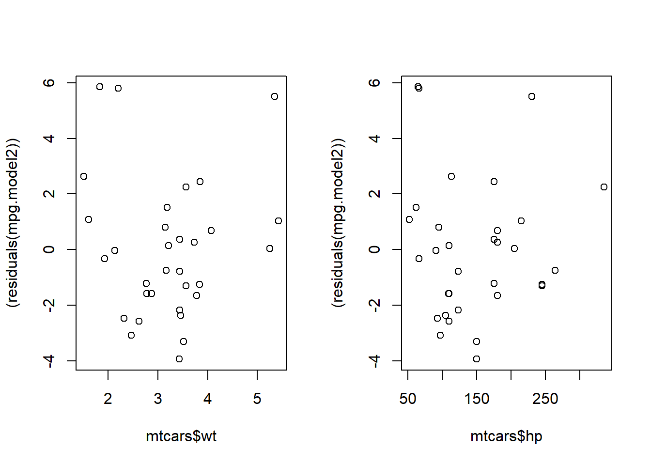
To check the linearity assumption, we plot the residuals of the model against the predictors of the model.
1par(mfrow=c(1,2))
2plot(mtcars$wt, (residuals(mpg.model2)))
3plot(mtcars$hp, (residuals(mpg.model2)))
1###add a loess curve
2scatter.smooth(mtcars$wt, residuals(mpg.model2))
3scatter.smooth(mtcars$hp, residuals(mpg.model2))
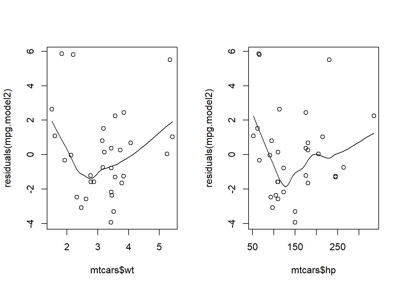
We don't want to see a trend in this plot. If it's random we've met the linearity assumption. At first, these plots look random. After adding a trend line, it's possible there might be an underlying pattern that wasn't captured in the model. You could try transforming the predictor variables to account for this.