Cleaning messy scripts and data
By Matt Brousil
The goal of this walkthrough is to look over some methods for cleaning and maintaining data and scripts. This will not be comprehensive for either topic, but contains some tips I've collected.
Data
Cleaned data is a wonderful thing. There are resources like Data Carpentry to provide crash courses in how to get started in doing data manipulation and management in R. Below are a few additional tips and tricks for cleaning up data that you may not have previously encountered.
1. Dealing with bad column names.
The csv below has the following column names in its raw form:
test date, which group?, value, group*value, "Notes"
How does R interpret those when read in?
1og_csv <- read.csv(file = "bad-header.csv")
2
3og_csv
 1##    test.date which.group. value group.value                 X.Notes.        lat
 2## 1      42370            A     1          A1 experimental, greenhouse -27.18648°
 3## 2      42371            A     5          A5 experimental, greenhouse -27.18648°
 4## 3      42371            B    75         B75        experimental, lab -27.18648°
 5## 4         NA            B     4          B4 experimental, greenhouse -27.18648°
 6## 5         NA            A     2          A2        experimental, lab -27.18648°
 7## 6      42370            A     1          A1 experimental, greenhouse -27.18648°
 8## 7      42373            A     1          A1        experimental, lab -27.18351°
 9## 8      42374            A   544        A544 experimental, greenhouse -27.18351°
10## 9      42375            B    45         B45        experimental, lab -27.18351°
11## 10     42370            A     1          A1 experimental, greenhouse -27.18351°
12##           long
13## 1  -109.43542°
14## 2  -109.43542°
15## 3  -109.43542°
16## 4  -109.43542°
17## 5  -109.43542°
18## 6  -109.43542°
19## 7  -109.44268°
20## 8  -109.44268°
21## 9  -109.44268°
22## 10 -109.44268°
There is a function working under-the-hood in R to make the crazy names of our
csv "valid." This is the function make.names(), which is referenced by
read.csv() by default. This is what happens if we turn it off:
1raw_csv <- read.csv(file = "bad-header.csv", check.names = F)
2
3raw_csv
 1##    test date which group? value group*value                  "Notes"        lat
 2## 1      42370            A     1          A1 experimental, greenhouse -27.18648°
 3## 2      42371            A     5          A5 experimental, greenhouse -27.18648°
 4## 3      42371            B    75         B75        experimental, lab -27.18648°
 5## 4         NA            B     4          B4 experimental, greenhouse -27.18648°
 6## 5         NA            A     2          A2        experimental, lab -27.18648°
 7## 6      42370            A     1          A1 experimental, greenhouse -27.18648°
 8## 7      42373            A     1          A1        experimental, lab -27.18351°
 9## 8      42374            A   544        A544 experimental, greenhouse -27.18351°
10## 9      42375            B    45         B45        experimental, lab -27.18351°
11## 10     42370            A     1          A1 experimental, greenhouse -27.18351°
12##           long
13## 1  -109.43542°
14## 2  -109.43542°
15## 3  -109.43542°
16## 4  -109.43542°
17## 5  -109.43542°
18## 6  -109.43542°
19## 7  -109.44268°
20## 8  -109.44268°
21## 9  -109.44268°
22## 10 -109.44268°
1str(raw_csv)
1## 'data.frame':	10 obs. of  7 variables:
2##  $ test date   : int  42370 42371 42371 NA NA 42370 42373 42374 42375 42370
3##  $ which group?: chr  "A" "A" "B" "B" ...
4##  $ value       : int  1 5 75 4 2 1 1 544 45 1
5##  $ group*value : chr  "A1" "A5" "B75" "B4" ...
6##  $ "Notes"     : chr  "experimental, greenhouse" "experimental, greenhouse" "experimental, lab" "experimental, greenhouse" ...
7##  $ lat         : chr  "-27.18648°" "-27.18648°" "-27.18648°" "-27.18648°" ...
8##  $ long        : chr  "-109.43542°" "-109.43542°" "-109.43542°" "-109.43542°" ...
If we want to start referencing those column names in our code it gets trickier, as we need to start quoting:
1raw_csv$`which group?`
1## [1] "A" "A" "B" "B" "A" "A" "A" "A" "B" "A"
There are a couple of ways to go about cleaning up the names of a messy file. We
can use make.names() as described above, which requires a vector of names
as input. Alternatively, we can use clean_names() from the janitor package.
clean_names() will take a data frame directly and return a new data frame
with tidy-looking names.
1make.names(names(raw_csv))
1## [1] "test.date"    "which.group." "value"        "group.value"  "X.Notes."
2## [6] "lat"          "long"
1clean_names(raw_csv) %>% names()
1## [1] "test_date"   "which_group" "value"       "group_value" "notes"
2## [6] "lat"         "long"
It also has a lot of options for changing case.
1clean_names(raw_csv, case = "upper_camel") %>% names()
1## [1] "TestDate"   "WhichGroup" "Value"      "GroupValue" "Notes"
2## [6] "Lat"        "Long"
We'll keep the tidier format:
1raw_csv <- clean_names(raw_csv)
2. One person's Excel dates are another person's usable data
Working with dates can be difficult at times, especially when importing them
from Excel. In some cases you will read in date data from Excel and find that
your dates have been converted to serial numbers such as this:
1raw_csv$test_date
1## [1] 42370 42371 42371 NA NA 42370 42373 42374 42375 42370
The janitor package comes in useful once again: We can use
excel_numeric_to_date() to convert these to dates we can use. Note that they
must be numeric.
1excel_numeric_to_date(as.numeric(raw_csv$test_date))
1##  [1] "2016-01-01" "2016-01-02" "2016-01-02" NA           NA
2##  [6] "2016-01-01" "2016-01-04" "2016-01-05" "2016-01-06" "2016-01-01"
1raw_csv$test_date <- excel_numeric_to_date(as.numeric(raw_csv$test_date))
3. Fill in NA values in a sequence of data
If you've entered data collected by hand, it isn't difficult to imagine a
situation where someone skips filling in rows that have identical data. For
example, we might know that the NA values in the date column below aren't truly
unknown. Perhaps our lab technician just didn't want to write the same date over
and over again.
1raw_csv
 1##     test_date which_group value group_value                    notes        lat
 2## 1  2016-01-01           A     1          A1 experimental, greenhouse -27.18648°
 3## 2  2016-01-02           A     5          A5 experimental, greenhouse -27.18648°
 4## 3  2016-01-02           B    75         B75        experimental, lab -27.18648°
 5## 4        <NA>           B     4          B4 experimental, greenhouse -27.18648°
 6## 5        <NA>           A     2          A2        experimental, lab -27.18648°
 7## 6  2016-01-01           A     1          A1 experimental, greenhouse -27.18648°
 8## 7  2016-01-04           A     1          A1        experimental, lab -27.18351°
 9## 8  2016-01-05           A   544        A544 experimental, greenhouse -27.18351°
10## 9  2016-01-06           B    45         B45        experimental, lab -27.18351°
11## 10 2016-01-01           A     1          A1 experimental, greenhouse -27.18351°
12##           long
13## 1  -109.43542°
14## 2  -109.43542°
15## 3  -109.43542°
16## 4  -109.43542°
17## 5  -109.43542°
18## 6  -109.43542°
19## 7  -109.44268°
20## 8  -109.44268°
21## 9  -109.44268°
22## 10 -109.44268°
In this case we can use the function na.locf() in the zoo package or the
fill() function in tidyr. Both of these functions will fill in missing values
in a data frame by moving either forward or backward through its values.
1na.locf(object = raw_csv$test_date)
1##  [1] "2016-01-01" "2016-01-02" "2016-01-02" "2016-01-02" "2016-01-02"
2##  [6] "2016-01-01" "2016-01-04" "2016-01-05" "2016-01-06" "2016-01-01"
fill() is more suited to working directly with a data frame:
1fill(data = raw_csv, test_date)
 1##     test_date which_group value group_value                    notes        lat
 2## 1  2016-01-01           A     1          A1 experimental, greenhouse -27.18648°
 3## 2  2016-01-02           A     5          A5 experimental, greenhouse -27.18648°
 4## 3  2016-01-02           B    75         B75        experimental, lab -27.18648°
 5## 4  2016-01-02           B     4          B4 experimental, greenhouse -27.18648°
 6## 5  2016-01-02           A     2          A2        experimental, lab -27.18648°
 7## 6  2016-01-01           A     1          A1 experimental, greenhouse -27.18648°
 8## 7  2016-01-04           A     1          A1        experimental, lab -27.18351°
 9## 8  2016-01-05           A   544        A544 experimental, greenhouse -27.18351°
10## 9  2016-01-06           B    45         B45        experimental, lab -27.18351°
11## 10 2016-01-01           A     1          A1 experimental, greenhouse -27.18351°
12##           long
13## 1  -109.43542°
14## 2  -109.43542°
15## 3  -109.43542°
16## 4  -109.43542°
17## 5  -109.43542°
18## 6  -109.43542°
19## 7  -109.44268°
20## 8  -109.44268°
21## 9  -109.44268°
22## 10 -109.44268°
4. Working with duplicate data
There are multiple ways to get duplicate rows from a data frame in R. get_dupes()
from janitor is straightforward. It also appends a new column to your input
data frame called dupe_count that indicates the number of rows duplicated for
each unique record.
1get_dupes(raw_csv)
1## No variable names specified - using all columns.
1##    test_date which_group value group_value                    notes        lat
2## 1 2016-01-01           A     1          A1 experimental, greenhouse -27.18648°
3## 2 2016-01-01           A     1          A1 experimental, greenhouse -27.18648°
4##          long dupe_count
5## 1 -109.43542°          2
6## 2 -109.43542°          2
We can also do something similar in base R using duplicated(). However, it
has fewer bells and whistles. We can see which rows are duplicates:
1duplicated(raw_csv)
1## [1] FALSE FALSE FALSE FALSE FALSE TRUE FALSE FALSE FALSE FALSE
Note that this includes one less duplicate than get_dupes(). This function
doesn't count the first entry as a duplicate, only the repeats.
1raw_csv[duplicated(raw_csv), ]
1##    test_date which_group value group_value                    notes        lat
2## 6 2016-01-01           A     1          A1 experimental, greenhouse -27.18648°
3##          long
4## 6 -109.43542°
5. Splitting rows based on a delimited value
You may run into a situation where you have a variable that has multiple values
within each of its rows. Perhaps this is a "Notes" column, for example. Depending
on the situation you'll either want to put these in their own rows or columns.
That is doable using separate() or separate_rows() from tidyr.
Use separate() to create new columns. We can specify the new column names with
into.
1separate(data = raw_csv, col = notes, into = c("type", "location"), sep = ", ")
 1##     test_date which_group value group_value         type   location        lat
 2## 1  2016-01-01           A     1          A1 experimental greenhouse -27.18648°
 3## 2  2016-01-02           A     5          A5 experimental greenhouse -27.18648°
 4## 3  2016-01-02           B    75         B75 experimental        lab -27.18648°
 5## 4        <NA>           B     4          B4 experimental greenhouse -27.18648°
 6## 5        <NA>           A     2          A2 experimental        lab -27.18648°
 7## 6  2016-01-01           A     1          A1 experimental greenhouse -27.18648°
 8## 7  2016-01-04           A     1          A1 experimental        lab -27.18351°
 9## 8  2016-01-05           A   544        A544 experimental greenhouse -27.18351°
10## 9  2016-01-06           B    45         B45 experimental        lab -27.18351°
11## 10 2016-01-01           A     1          A1 experimental greenhouse -27.18351°
12##           long
13## 1  -109.43542°
14## 2  -109.43542°
15## 3  -109.43542°
16## 4  -109.43542°
17## 5  -109.43542°
18## 6  -109.43542°
19## 7  -109.44268°
20## 8  -109.44268°
21## 9  -109.44268°
22## 10 -109.44268°
Alternatively, you can use separate_rows() to create new rows from the data
instead.
1separate_rows(data = raw_csv, notes, sep = ", ") %>% head()
1## # A tibble: 6 x 7
2##   test_date  which_group value group_value notes        lat        long
3##   <date>     <chr>       <int> <chr>       <chr>        <chr>      <chr>
4## 1 2016-01-01 A               1 A1          experimental -27.18648° -109.43542°
5## 2 2016-01-01 A               1 A1          greenhouse   -27.18648° -109.43542°
6## 3 2016-01-02 A               5 A5          experimental -27.18648° -109.43542°
7## 4 2016-01-02 A               5 A5          greenhouse   -27.18648° -109.43542°
8## 5 2016-01-02 B              75 B75         experimental -27.18648° -109.43542°
9## 6 2016-01-02 B              75 B75         lab          -27.18648° -109.43542°
Scripts
So now your data is beautiful. But your script isn't! It is easy to treat a script as something that only needs to run, and doesn't need to be polished. Often this will work, too. We can write scripts that may be hard to read but will run if we ask them.
If you're trying to make a reproducible analysis a script won't be very useful for the next user if they can't interpret it.
One way to ensure some readability in scripts is to follow a style guide. For example, the tidyverse provides one here: https://style.tidyverse.org/
This style guide goes into many specifics, which I won't rewrite here, but for example:
Names of objects should use underscores, not periods.
1hour_sequence <- seq(from = 1, to = 24, by = 1)
2
3# NOT
4
5hour.sequence <- seq(from = 1, to = 24, by = 1)
Operators should typically have spaces on either side.
1filter(iris, Sepal.Width >= 3)
2
3# NOT
4
5filter(iris, Sepal.Width>=3)
Long lines (> 80 characters) are bad news. Avoid letting the code run longer than this on one line.
1iris %>%
2  filter(Sepal.Width >= 3) %>%
3  select(Sepal.Width, Species) %>%
4  group_by(Species) %>%
5  summarise(mean = mean(Sepal.Width))
6
7# NOT
8
9iris %>% filter(Sepal.Width >= 3) %>% select(Sepal.Width, Species) %>% group_by(Species) %>% summarise(mean = mean(Sepal.Width))
Despite your best efforts you may find yourself missing some of the style points
once you've finished a script. Have no fear! You can use the lintr package
to check your script for style automatically.
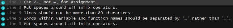
1lint("example_script.R")
Where "example_script.R" looks like
1#This is an example script with some messy code
2
3iris.sepal=iris %>% select(Sepal.Length, Sepal.Width, Species)
4
5iris.petal.means <- iris %>% select(Petal.Length, Petal.Width, Species) %>% group_by(Species) %>% summarise(mean=mean(Petal.Length))
and the lintr output is
If you have specific aspects of style that you'd like to check, you can specify
specific linters from within the lint() call. Available linters can be viewed
using ?linters()