Clustering in R

Oct 2, 2019 · 5 min read · clustering ·

By Enrique Jimenez

 1library(ggplot2)
 2
 3## Warning: package 'ggplot2' was built under R version 3.5.3
 4
 5library(ggpubr)
 6
 7## Warning: package 'ggpubr' was built under R version 3.5.3
 8
 9library(cluster)
10
11## Warning: package 'cluster' was built under R version 3.5.3
12
13library(factoextra)
14
15## Warning: package 'factoextra' was built under R version 3.5.3
16
17library(NbClust)
18
19## Warning: package 'NbClust' was built under R version 3.5.2
20
21library(tidyLPA)
22
23## Warning: package 'tidyLPA' was built under R version 3.5.3

What is clustering?

Clustering or cluster analysis is the task of dividing a data set into groups of similar individuals. When clustering we generally want our groups to be similar within (individuals within a group are as similar as possible) and different between (the individuals from different groups are as different as possible).

k-means Clustering

k-means clustering is one of the simplest and most commonly used clustering algorithms. It works by iteratively assigning individuals to one of k centroids (means) and recalibrating the locations of the menas based on the groups created.

k-means example

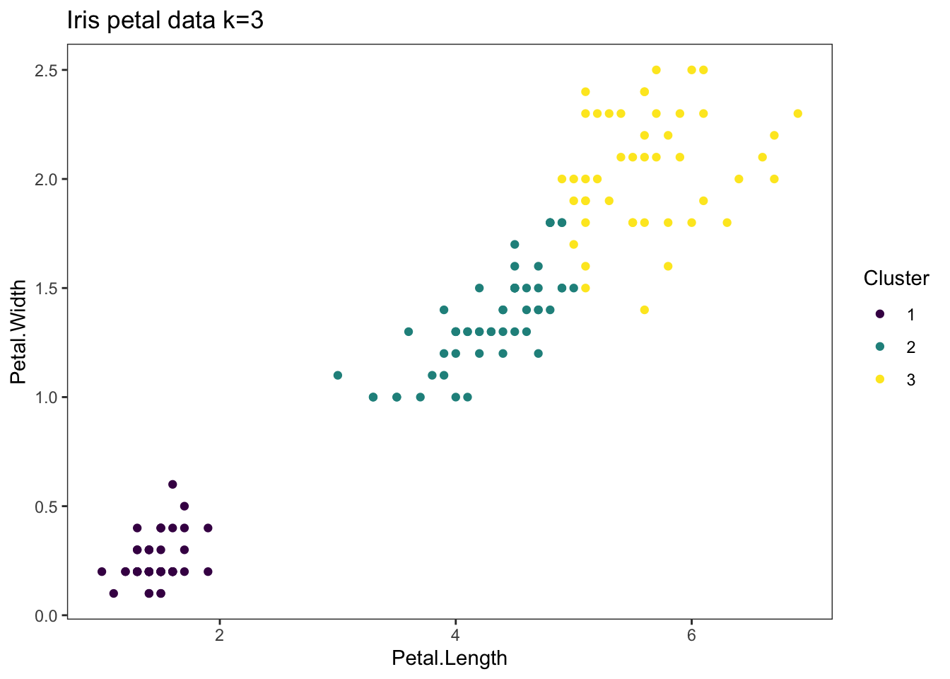
We will use the classic Fisher's iris dataset mostly because Fisher was cool. However, for simplicity, we will use only the petal measurements.

 1  data("iris")
 2  petals_kmeans<-iris[,3:5]
 3  head(petals_kmeans)
 4
 5##   Petal.Length Petal.Width Species
 6## 1          1.4         0.2  setosa
 7## 2          1.4         0.2  setosa
 8## 3          1.3         0.2  setosa
 9## 4          1.5         0.2  setosa
10## 5          1.4         0.2  setosa
11## 6          1.7         0.4  setosa
12
13  set.seed(23)
14  petals_kmeans_3<-kmeans(iris[,3:4], centers = 3)
15  petals_kmeans$k3<-petals_kmeans_3$cluster
16  head(petals_kmeans)
17
18##   Petal.Length Petal.Width Species k3
19## 1          1.4         0.2  setosa  3
20## 2          1.4         0.2  setosa  3
21## 3          1.3         0.2  setosa  3
22## 4          1.5         0.2  setosa  3
23## 5          1.4         0.2  setosa  3
24## 6          1.7         0.4  setosa  3
25
26  iris_plot_k3<-ggplot(petals_kmeans) +
27  geom_point(aes(x=Petal.Length, y=Petal.Width, colour=as.factor(k3)), data=petals_kmeans) +
28  theme_bw() +
29  theme(panel.grid = element_blank()) +
30  scale_color_viridis_d() +
31  ggtitle("Iris petal data k=3") +
32  labs(colour="Cluster")
33
34  iris_plot_k3

 1  set.seed(23)
 2  petals_kmeans_4<-kmeans(iris[,3:4], centers = 4)
 3  petals_kmeans$k4<-petals_kmeans_4$cluster
 4
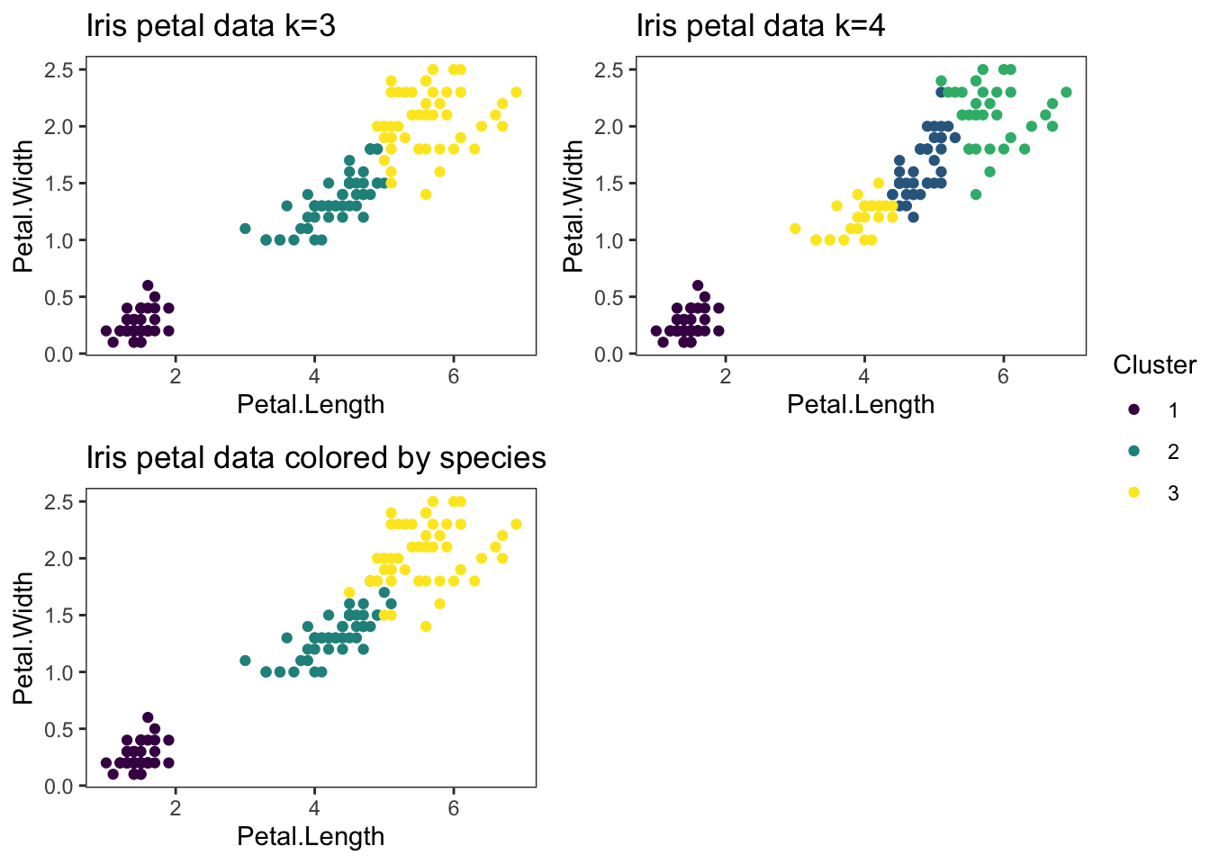
 5  iris_plot_k4<-ggplot(petals_kmeans) +
 6  geom_point(aes(x=Petal.Length, y=Petal.Width, colour=as.factor(k4)), data=petals_kmeans) +
 7  theme_bw() +
 8  theme(panel.grid = element_blank()) +
 9  scale_color_viridis_d() +
10  ggtitle("Iris petal data k=4") +
11  labs(colour = "Cluster")
12
13  iris_plot_k4

1  iris_plot_species<-ggplot(petals_kmeans) +
2  geom_point(aes(x=Petal.Length, y=Petal.Width, colour=as.factor(Species)), data=petals_kmeans) +
3  theme_bw() +
4  theme(panel.grid = element_blank()) +
5  scale_color_viridis_d() +
6  ggtitle("Iris petal data colored by species") +
7  labs(colour = "Species")
8
9  iris_plot_species

1  final_figure <- ggarrange(plotlist = list(iris_plot_k3, iris_plot_k4, iris_plot_species),
2          common.legend = TRUE,
3          legend = "right")
4  final_figure

Other simple clustering algorithms

K-medoids algorithm or PAM
Heirarchical clustering

Model evaluation

One of the difficulties in using k-means clustering and other similar clustering algorithms is selecting the number of clusters.

Determining the number of clusters

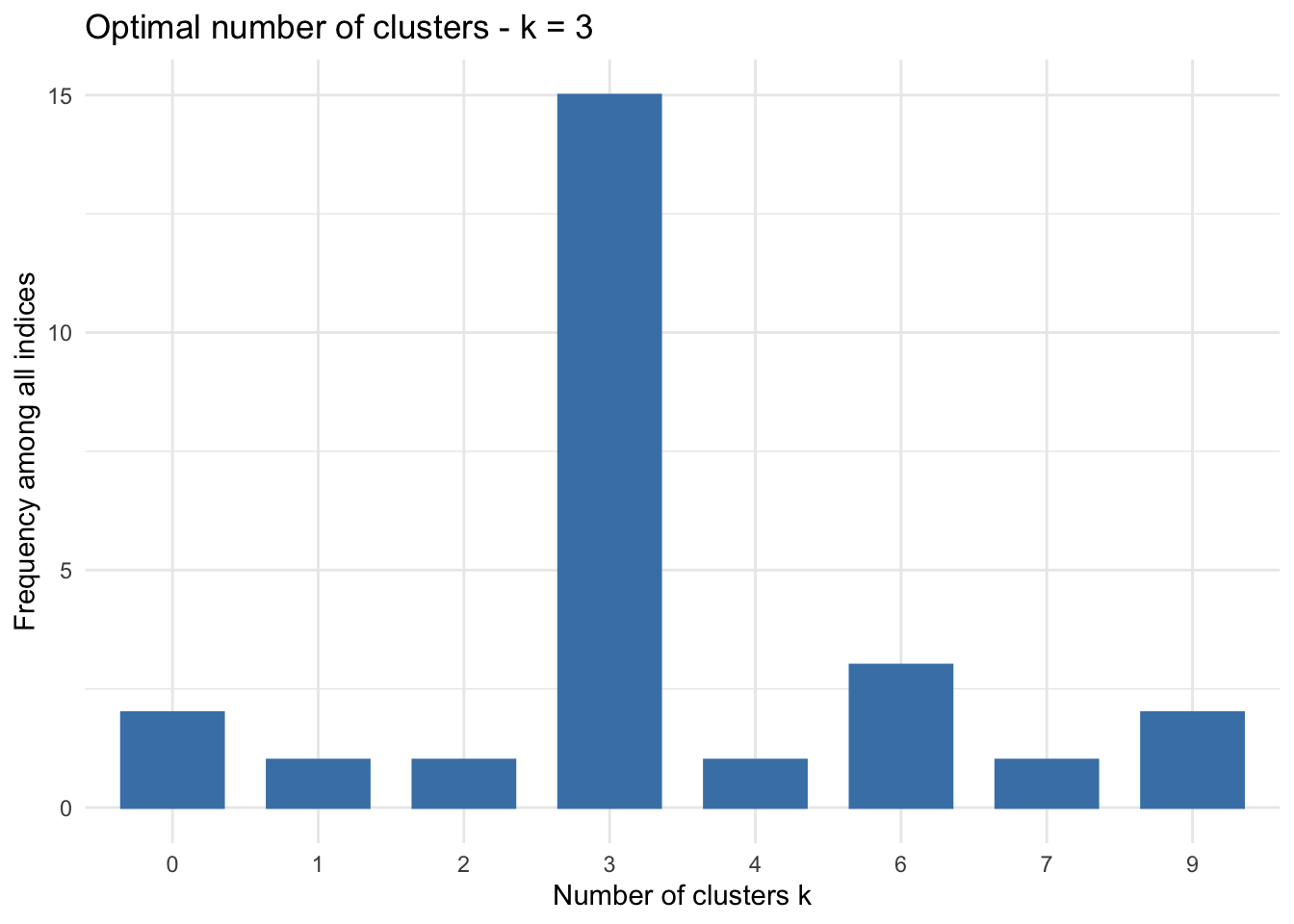
There are a large number of measurements that help determine the ideal number of clusters into which a set of data should be split. NbClust provides a function to leverage this field of indices.

 1nb<-NbClust(iris[3:4], distance = 'euclidean', min.nc = 2, max.nc = 9, method = "complete", index= "all",)
 2
 3  fviz_nbclust(nb) + theme_minimal()
 4
 5## Among all indices:
 6## ===================
 7## * 2 proposed  0 as the best number of clusters
 8## * 1 proposed  1 as the best number of clusters
 9## * 1 proposed  2 as the best number of clusters
10## * 15 proposed  3 as the best number of clusters
11## * 1 proposed  4 as the best number of clusters
12## * 3 proposed  6 as the best number of clusters
13## * 1 proposed  7 as the best number of clusters
14## * 2 proposed  9 as the best number of clusters
15##
16## Conclusion
17## =========================
18## * According to the majority rule, the best number of clusters is  3 .

Silhouette Coefficient

The Silhouette Coefficient uses the distances between individuals in the same cluster and their average distance to every individual in the nearest class to evalueate a clustering run. The larger the number, the better the clustering.

1  sil_k3<-silhouette(petals_kmeans_3$cluster, dist(petals_kmeans[1:2]))
2  sil_k4<-silhouette(petals_kmeans_4$cluster, dist(petals_kmeans[1:2]))
3  sil_plot_k3<-fviz_silhouette(sil_k3, print.summary = FALSE) +
4    scale_color_viridis_d()
5  sil_plot_k4<-fviz_silhouette(sil_k4, print.summary = FALSE) +
6    scale_color_viridis_d()
7  ggarrange(plotlist = list(sil_plot_k3, sil_plot_k4),
8          common.legend = FALSE,
9          legend = FALSE)

Other clustering evaluation methods

Calinski-Harabasz Index
Davies-Bouldin Index
Dunn Index

Model based clustering

An alternative to the traditional clustering methods is model based clustering, which allows for the use of likelihood-based evaluation of the models.

Latent Profile Analysis

Latent Profile Analysis (LPA) is one version of what are called latent variable models. Broadly speaking latent variable models are ones where an unobserved (or latent) variable is modeled from observed or manifest variables. LPA is the latent variable model that plays the function of a cluster analysis. In the case of LPA, the latent variable is categorical, representing the classes or clusters in which the data is binned and the observed variables are continuous. Therefore, LPA acts as a clustering model for continuous observed variables. Within the framework of latent variable models there is also a clustering model for categorical observed variables: Latent class analysis.

Here we'll use library(tidyLPA) to run an LPA on the petal data.

 1  LPA_1.5<-estimate_profiles(petals_kmeans[,1:2], 1:7)
 2
 3## Warning:
 4## One or more analyses resulted in warnings! Examine these analyses carefully: model_1_class_7
 5
 6  LPA_1.5
 7
 8## tidyLPA analysis using mclust:
 9##
10##  Model Classes AIC    BIC    Entropy prob_min prob_max n_min n_max BLRT_p
11##  1     1       946.40 958.45 1.00    1.00     1.00     1.00  1.00
12##  1     2       623.59 644.67 0.98    0.99     1.00     0.33  0.67  0.01
13##  1     3       439.46 469.56 0.96    0.97     1.00     0.32  0.35  0.01
14##  1     4       399.78 438.92 0.92    0.89     1.00     0.18  0.33  0.01
15##  1     5       385.14 433.31 0.93    0.88     1.00     0.05  0.33  0.01
16##  1     6       338.55 395.76 0.95    0.90     1.00     0.05  0.33  0.01
17##  1     7       343.97 410.20 0.94    0.46     0.99     0.01  0.33  0.57
18
19  ggplot(get_data(LPA_1.5)[which(get_data(LPA_1.5)$classes_number==3),]) +
20    geom_point(aes(x = Petal.Length, y=Petal.Width, colour=as.factor(Class))) +
21    theme_bw() +
22    theme(panel.grid = element_blank()) +
23    scale_color_viridis_d() +
24    ggtitle("Iris petal data LPA 5") +
25    labs(colour = "Class")

One thing to keep in mind is that, as a model-based method, LPA is tied to a series of assumptions. One of these assumptions refers to the structure of the covariance matrix of the observed variables, which can drastically affect the fit of LPA models.