Introduction to R - A Roadmap
Author: Alli N. Cramer
This is an attempt to orient you around R. To give you a roadmap of sorts to help you find your way when learning R. The following text will show you:
- What R is
- What R studio is
- How to do basic math in R
- How to add, save, and bring in data
- How to read basic R syntax
- How to make a linear model and a basic plot
- How to add packages
- What a dplyr pipe is
- How to plot with ggplot
This is, of course, just the tip of the iceberg as far as R goes but hopefully this orients you so that you can follow along in future R sessions.
Once you've mastered the skills in this post I suggest you download and do the Lab 1 Walkthrough using the Floral Diversity Dataset created by our very own Rachel Olsson. This is an in-depth walk through and a great way to familiarize yourself with R terms and capabilities.
What is R?
R is a free software for stats. It also is useful for data cleaning and making graphics. R runs in what is called the "console". If you open R (not in R studio) you will see a simple box for code input, perhaps with some red or blue colors. This is basic R.
What is RStudio?
RStudio is a wrapper for R, or an IDE (integrated development environment). It runs the R Console within it, normally at the bottom left. The top right is the script pane.The Environment on the top right shows you what data R is remembering and keeping track of. The bottom right pane has help (super useful), shows plots, lets you point and click to install packages, and more.
The Scripte Pane lets you write scripts, but not necessarily have R do anything until you send the code to the R Console. To send information from scripts to the console, you can highlight the script and press the green "run" arrow at the top right of the script pane. You can also use some short cuts to sent code back and forth from the console and script pane :
Some shortcuts for RStudio:
Highlight the code chunk, or run whatever line your cursor is on.
- ctrl + Enter (shortcut to run code)
- ctrl + 1 (go to script pane)
- ctrl + 2 (go to R Console)
- alt + - (shortcut to make "<-" symbol)
Using Basic R
R as a calculator
First, lets explore R like any simple computer program - as a calculator. If we simply type "2+3" into the script pane and then send it to the R Console:
12+3
2
3## [1] 5
We can see that R understood the code, and gave us the right answer. We can also see however, by looking at the Environment pane on the top right, that R doesn't remember this data. To do that we will need create an object (something for R to keep track of) and assign a value.
Assign values to objects
To assign a value we use a "<-" symbol and a name. lets use x and y. We can also assign a value to the answer, lets use z:
1#use alt + - for arrow shortcut
2x <- 2
3
4y <- 3
5
6z <- x + y
We can see that R now keeps track of these objects by looking in the environment:

Working with Data
Using R as a calculator is great, but lets work with some data. We will start by working with built in data. This is data that comes pre-loaded in R to assist teaching. We will work with the "iris" data set. Other good built in data sets, which work with this lesson, are "AirPassengers" and "ChickWeight". There is also the BACups data set, a data set of bronze age cup dimensions. To see the iris data set, type "iris".
1#built in data
2iris
3
4## Sepal.Length Sepal.Width Petal.Length Petal.Width Species
5## 1 5.1 3.5 1.4 0.2 setosa
6## 2 4.9 3.0 1.4 0.2 setosa
7## 3 4.7 3.2 1.3 0.2 setosa
8## 4 4.6 3.1 1.5 0.2 setosa
9## 5 5.0 3.6 1.4 0.2 setosa
10## 6 5.4 3.9 1.7 0.4 setosa
11## 7 4.6 3.4 1.4 0.3 setosa
12## 8 5.0 3.4 1.5 0.2 setosa
13## 9 4.4 2.9 1.4 0.2 setosa
14## 10 4.9 3.1 1.5 0.1 setosa
15## 11 5.4 3.7 1.5 0.2 setosa
16## 12 4.8 3.4 1.6 0.2 setosa
17## 13 4.8 3.0 1.4 0.1 setosa
18## 14 4.3 3.0 1.1 0.1 setosa
19## 15 5.8 4.0 1.2 0.2 setosa
20## 16 5.7 4.4 1.5 0.4 setosa
21## 17 5.4 3.9 1.3 0.4 setosa
22## 18 5.1 3.5 1.4 0.3 setosa
23## 19 5.7 3.8 1.7 0.3 setosa
24## 20 5.1 3.8 1.5 0.3 setosa
25## 21 5.4 3.4 1.7 0.2 setosa
26## 22 5.1 3.7 1.5 0.4 setosa
27## 23 4.6 3.6 1.0 0.2 setosa
28## 24 5.1 3.3 1.7 0.5 setosa
29## 25 4.8 3.4 1.9 0.2 setosa
30## 26 5.0 3.0 1.6 0.2 setosa
31## 27 5.0 3.4 1.6 0.4 setosa
32## 28 5.2 3.5 1.5 0.2 setosa
33## 29 5.2 3.4 1.4 0.2 setosa
34## 30 4.7 3.2 1.6 0.2 setosa
35## 31 4.8 3.1 1.6 0.2 setosa
36## 32 5.4 3.4 1.5 0.4 setosa
37## 33 5.2 4.1 1.5 0.1 setosa
38## 34 5.5 4.2 1.4 0.2 setosa
39## 35 4.9 3.1 1.5 0.2 setosa
40## 36 5.0 3.2 1.2 0.2 setosa
41## 37 5.5 3.5 1.3 0.2 setosa
42## 38 4.9 3.6 1.4 0.1 setosa
43## 39 4.4 3.0 1.3 0.2 setosa
44## 40 5.1 3.4 1.5 0.2 setosa
45## 41 5.0 3.5 1.3 0.3 setosa
46## 42 4.5 2.3 1.3 0.3 setosa
47## 43 4.4 3.2 1.3 0.2 setosa
48## 44 5.0 3.5 1.6 0.6 setosa
49## 45 5.1 3.8 1.9 0.4 setosa
50## 46 4.8 3.0 1.4 0.3 setosa
51## 47 5.1 3.8 1.6 0.2 setosa
52## 48 4.6 3.2 1.4 0.2 setosa
53## 49 5.3 3.7 1.5 0.2 setosa
54## 50 5.0 3.3 1.4 0.2 setosa
55## 51 7.0 3.2 4.7 1.4 versicolor
56## 52 6.4 3.2 4.5 1.5 versicolor
57## 53 6.9 3.1 4.9 1.5 versicolor
58## 54 5.5 2.3 4.0 1.3 versicolor
59## 55 6.5 2.8 4.6 1.5 versicolor
60## 56 5.7 2.8 4.5 1.3 versicolor
61## 57 6.3 3.3 4.7 1.6 versicolor
62## 58 4.9 2.4 3.3 1.0 versicolor
63## 59 6.6 2.9 4.6 1.3 versicolor
64## 60 5.2 2.7 3.9 1.4 versicolor
65## 61 5.0 2.0 3.5 1.0 versicolor
66## 62 5.9 3.0 4.2 1.5 versicolor
67## 63 6.0 2.2 4.0 1.0 versicolor
68## 64 6.1 2.9 4.7 1.4 versicolor
69## 65 5.6 2.9 3.6 1.3 versicolor
70## 66 6.7 3.1 4.4 1.4 versicolor
71## 67 5.6 3.0 4.5 1.5 versicolor
72## 68 5.8 2.7 4.1 1.0 versicolor
73## 69 6.2 2.2 4.5 1.5 versicolor
74## 70 5.6 2.5 3.9 1.1 versicolor
75## 71 5.9 3.2 4.8 1.8 versicolor
76## 72 6.1 2.8 4.0 1.3 versicolor
77## 73 6.3 2.5 4.9 1.5 versicolor
78## 74 6.1 2.8 4.7 1.2 versicolor
79## 75 6.4 2.9 4.3 1.3 versicolor
80## 76 6.6 3.0 4.4 1.4 versicolor
81## 77 6.8 2.8 4.8 1.4 versicolor
82## 78 6.7 3.0 5.0 1.7 versicolor
83## 79 6.0 2.9 4.5 1.5 versicolor
84## 80 5.7 2.6 3.5 1.0 versicolor
85## 81 5.5 2.4 3.8 1.1 versicolor
86## 82 5.5 2.4 3.7 1.0 versicolor
87## 83 5.8 2.7 3.9 1.2 versicolor
88## 84 6.0 2.7 5.1 1.6 versicolor
89## 85 5.4 3.0 4.5 1.5 versicolor
90## 86 6.0 3.4 4.5 1.6 versicolor
91## 87 6.7 3.1 4.7 1.5 versicolor
92## 88 6.3 2.3 4.4 1.3 versicolor
93## 89 5.6 3.0 4.1 1.3 versicolor
94## 90 5.5 2.5 4.0 1.3 versicolor
95## 91 5.5 2.6 4.4 1.2 versicolor
96## 92 6.1 3.0 4.6 1.4 versicolor
97## 93 5.8 2.6 4.0 1.2 versicolor
98## 94 5.0 2.3 3.3 1.0 versicolor
99## 95 5.6 2.7 4.2 1.3 versicolor
100## 96 5.7 3.0 4.2 1.2 versicolor
101## 97 5.7 2.9 4.2 1.3 versicolor
102## 98 6.2 2.9 4.3 1.3 versicolor
103## 99 5.1 2.5 3.0 1.1 versicolor
104## 100 5.7 2.8 4.1 1.3 versicolor
105## 101 6.3 3.3 6.0 2.5 virginica
106## 102 5.8 2.7 5.1 1.9 virginica
107## 103 7.1 3.0 5.9 2.1 virginica
108## 104 6.3 2.9 5.6 1.8 virginica
109## 105 6.5 3.0 5.8 2.2 virginica
110## 106 7.6 3.0 6.6 2.1 virginica
111## 107 4.9 2.5 4.5 1.7 virginica
112## 108 7.3 2.9 6.3 1.8 virginica
113## 109 6.7 2.5 5.8 1.8 virginica
114## 110 7.2 3.6 6.1 2.5 virginica
115## 111 6.5 3.2 5.1 2.0 virginica
116## 112 6.4 2.7 5.3 1.9 virginica
117## 113 6.8 3.0 5.5 2.1 virginica
118## 114 5.7 2.5 5.0 2.0 virginica
119## 115 5.8 2.8 5.1 2.4 virginica
120## 116 6.4 3.2 5.3 2.3 virginica
121## 117 6.5 3.0 5.5 1.8 virginica
122## 118 7.7 3.8 6.7 2.2 virginica
123## 119 7.7 2.6 6.9 2.3 virginica
124## 120 6.0 2.2 5.0 1.5 virginica
125## 121 6.9 3.2 5.7 2.3 virginica
126## 122 5.6 2.8 4.9 2.0 virginica
127## 123 7.7 2.8 6.7 2.0 virginica
128## 124 6.3 2.7 4.9 1.8 virginica
129## 125 6.7 3.3 5.7 2.1 virginica
130## 126 7.2 3.2 6.0 1.8 virginica
131## 127 6.2 2.8 4.8 1.8 virginica
132## 128 6.1 3.0 4.9 1.8 virginica
133## 129 6.4 2.8 5.6 2.1 virginica
134## 130 7.2 3.0 5.8 1.6 virginica
135## 131 7.4 2.8 6.1 1.9 virginica
136## 132 7.9 3.8 6.4 2.0 virginica
137## 133 6.4 2.8 5.6 2.2 virginica
138## 134 6.3 2.8 5.1 1.5 virginica
139## 135 6.1 2.6 5.6 1.4 virginica
140## 136 7.7 3.0 6.1 2.3 virginica
141## 137 6.3 3.4 5.6 2.4 virginica
142## 138 6.4 3.1 5.5 1.8 virginica
143## 139 6.0 3.0 4.8 1.8 virginica
144## 140 6.9 3.1 5.4 2.1 virginica
145## 141 6.7 3.1 5.6 2.4 virginica
146## 142 6.9 3.1 5.1 2.3 virginica
147## 143 5.8 2.7 5.1 1.9 virginica
148## 144 6.8 3.2 5.9 2.3 virginica
149## 145 6.7 3.3 5.7 2.5 virginica
150## 146 6.7 3.0 5.2 2.3 virginica
151## 147 6.3 2.5 5.0 1.9 virginica
152## 148 6.5 3.0 5.2 2.0 virginica
153## 149 6.2 3.4 5.4 2.3 virginica
154## 150 5.9 3.0 5.1 1.8 virginica
Iris is relatively small dataset, but it is large enough to be annoying to look at. Imagine if it was even bigger! To deal with this, we can look at the top or the bottom of the data with head() and tail() commands.
 1#look at top of data(defaults to first 6 rows)
 2head(iris)
 3
 4##   Sepal.Length Sepal.Width Petal.Length Petal.Width Species
 5## 1          5.1         3.5          1.4         0.2  setosa
 6## 2          4.9         3.0          1.4         0.2  setosa
 7## 3          4.7         3.2          1.3         0.2  setosa
 8## 4          4.6         3.1          1.5         0.2  setosa
 9## 5          5.0         3.6          1.4         0.2  setosa
10## 6          5.4         3.9          1.7         0.4  setosa
11
12#look at tail of data (defaults to last 6 rows)
13tail(iris)
14
15##     Sepal.Length Sepal.Width Petal.Length Petal.Width   Species
16## 145          6.7         3.3          5.7         2.5 virginica
17## 146          6.7         3.0          5.2         2.3 virginica
18## 147          6.3         2.5          5.0         1.9 virginica
19## 148          6.5         3.0          5.2         2.0 virginica
20## 149          6.2         3.4          5.4         2.3 virginica
21## 150          5.9         3.0          5.1         1.8 virginica
22
23#can change the number of rows we see
24head(iris, n = 10)
25
26##    Sepal.Length Sepal.Width Petal.Length Petal.Width Species
27## 1           5.1         3.5          1.4         0.2  setosa
28## 2           4.9         3.0          1.4         0.2  setosa
29## 3           4.7         3.2          1.3         0.2  setosa
30## 4           4.6         3.1          1.5         0.2  setosa
31## 5           5.0         3.6          1.4         0.2  setosa
32## 6           5.4         3.9          1.7         0.4  setosa
33## 7           4.6         3.4          1.4         0.3  setosa
34## 8           5.0         3.4          1.5         0.2  setosa
35## 9           4.4         2.9          1.4         0.2  setosa
36## 10          4.9         3.1          1.5         0.1  setosa
Changing the Data
We're going to add a column to iris, so the first thing we need to do is rename iris. This is a data best practice (NEVER CHANGE RAW DATA!) and will let R keep track of what we're doing. In this case lets call our new data "ire".
1#assign the built in data to a new object name
2#so that we can change things about it
3#without changing the underlying data
4ire <- iris
Now, lets add an area column. R syntax for columns is the "$". The dataset name is on the left, the column name on the right. In this case, we are going to make an Area column. First, we tell R that we are making an area column by typing the new column information on the left of the assign arrow, then the math to make the column on the right.
1#adding and "area" column to iris
2# $ references a column in a data frame
3
4ire$Sepal.Area <- ire$Sepal.Length * ire$Sepal.Width
Lets look at these new data:
 1#top few rows
 2head(ire)
 3
 4##   Sepal.Length Sepal.Width Petal.Length Petal.Width Species Sepal.Area
 5## 1          5.1         3.5          1.4         0.2  setosa      17.85
 6## 2          4.9         3.0          1.4         0.2  setosa      14.70
 7## 3          4.7         3.2          1.3         0.2  setosa      15.04
 8## 4          4.6         3.1          1.5         0.2  setosa      14.26
 9## 5          5.0         3.6          1.4         0.2  setosa      18.00
10## 6          5.4         3.9          1.7         0.4  setosa      21.06
11
12#structure of the dataset
13str(ire)
14
15## 'data.frame':    150 obs. of  6 variables:
16##  $ Sepal.Length: num  5.1 4.9 4.7 4.6 5 5.4 4.6 5 4.4 4.9 ...
17##  $ Sepal.Width : num  3.5 3 3.2 3.1 3.6 3.9 3.4 3.4 2.9 3.1 ...
18##  $ Petal.Length: num  1.4 1.4 1.3 1.5 1.4 1.7 1.4 1.5 1.4 1.5 ...
19##  $ Petal.Width : num  0.2 0.2 0.2 0.2 0.2 0.4 0.3 0.2 0.2 0.1 ...
20##  $ Species     : Factor w/ 3 levels "setosa","versicolor",..: 1 1 1 1 1 1 1 1 1 1 ...
21##  $ Sepal.Area  : num  17.8 14.7 15 14.3 18 ...
Saving Data
Now we will save the data. First, we need to determine where the file will go. By default it will go to the current directory, so lets check where we currently are, then change it to where we want it to go:
1#where is the file going!?!?!?
2
3#where am I currently?
4getwd()
5
6#change location to new file path, if necessary :
7
8setwd("your_file_path/full_path")
Now, we save the data as a .csv file. For any R command, we can either specify the exact values of variables using the equals sign, or we can type information in the assumed order. See the help section for various commands to learn the assumed order. Knowing that this is possible can help you follow along when watching or reading other's R code.
1#write out data
2write.csv(x = ire, file = "Irisdata.csv", row.names = FALSE)
3
4#writing out the data using the same command, but the "assumed order", so no "x = " etc. needed
5write.csv(ire, "Irisdata2.csv")
To bring in the data, we use the read.csv() command. Remember to assign the data to an object, or R won't be able to do anything with it!
 1#bringing in data
 2#we need to assign to an object so we can use the dataset
 3dat <- read.csv("Irisdata.csv")
 4
 5head(dat)
 6
 7##   Sepal.Length Sepal.Width Petal.Length Petal.Width Species Sepal.Area
 8## 1          5.1         3.5          1.4         0.2  setosa      17.85
 9## 2          4.9         3.0          1.4         0.2  setosa      14.70
10## 3          4.7         3.2          1.3         0.2  setosa      15.04
11## 4          4.6         3.1          1.5         0.2  setosa      14.26
12## 5          5.0         3.6          1.4         0.2  setosa      18.00
13## 6          5.4         3.9          1.7         0.4  setosa      21.06
Now, lets clean up our workspace and remove the old objects we don't care about. Currently, R is remembering all of them and it takes up valuable memory on our computer
 1#remove object we don't care about using rm()
 2rm(x, y, z, ire)
 3
 4#check what objects remain using ls()
 5ls()
 6
 7##  [1] "answer"             "d"                  "dat"
 8##  [4] "mod"                "nonsensecolumndata" "ob"
 9##  [7] "ob1"                "p"                  "p1"
10## [10] "pg"
Modeling and Visualization
This is the fun part!
Lets make a basic plot by plotting the new Area column against Petal Width
1#plotting and a simple model
2#plot(y~x, data)
3
4plot(Sepal.Area ~ Petal.Width, data = dat)

1#can plot with or without color.
2p <- plot(Sepal.Area ~ Petal.Width, data = dat, col = Species)

1#there are lots of plot options - see help section for more.
Plots are cool, but what about models? Lets do a simple linear regression using the lm() command, or "linear model" command. we are going to name our linear model "mod".
 1#linear model
 2mod <- lm(Sepal.Area ~ Petal.Width, data = dat)
 3mod
 4
 5##
 6## Call:
 7## lm(formula = Sepal.Area ~ Petal.Width, data = dat)
 8##
 9## Coefficients:
10## (Intercept)  Petal.Width
11##      15.872        1.627
12
13#how to see p-values etc.
14summary(mod)
15
16##
17## Call:
18## lm(formula = Sepal.Area ~ Petal.Width, data = dat)
19##
20## Residuals:
21##     Min      1Q  Median      3Q     Max
22## -7.4986 -2.0099  0.0646  1.9034 10.8946
23##
24## Coefficients:
25##             Estimate Std. Error t value Pr(>|t|)
26## (Intercept)  15.8718     0.4784  33.176  < 2e-16 ***
27## Petal.Width   1.6268     0.3370   4.828 3.41e-06 ***
28## ---
29## Signif. codes:  0 '***' 0.001 '**' 0.01 '*' 0.05 '.' 0.1 ' ' 1
30##
31## Residual standard error: 3.135 on 148 degrees of freedom
32## Multiple R-squared:  0.136,  Adjusted R-squared:  0.1302
33## F-statistic: 23.31 on 1 and 148 DF,  p-value: 3.41e-06
Now, lets add this linear model to the plot. To do this in basic R (which is what we've used so far) we use the abline() command. Normally R doesn't care about spaces - all that matters is running the code to the next parentheses. abline() is different and * **needs* _to be right underneath the plot command_.
1#add model line to the plot
2plot(Sepal.Area ~ Petal.Width, data = dat, col = Species)
3abline(mod)

Ooooooo! A fancy plot with a linear model.
Gettin' fancy with packages
Up until this point we have only used the base capabilities of R. This is like painting with only black and white - there are so many more colors! To get more colors, or capabilities, from R we need to use packages.
Packages are sets of algorithms, functions, or mini-programs that can be added to R. These packages range from statistically focused to graphics focused. As R is open source, packages come from R users within the community. Packages that have passed a set of quality checks are hosted on the "CRAN", the same place you downloaded R from. These packages are more reliable than others, however you can also get packages off of places like github, from zip files, or even write your own.
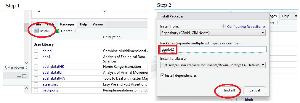
Lets install two packages, dplyr and ggplot, to explore our data more. We can do this two ways, by using the install.packages() command, or by point and click.
1#install packages using install.packages()
2
3install.packages("dplyr")
Installing by Point and Click:
To use the functions within the packages, we need to tell R to use the packages using library(). When doing this, you may get some warnings. Read the warnings to understand what is happening. Most of the warnings are simply telling you that some commands are called the same things within R. If you load a package using library and it has functions with the same names as previously loaded packages, the default function with that name will become the most recently loaded function. See the example below with the "filter" function when we load dplyr. The stats package (which comes pre-loaded) also has a filter function:
1#to use functions in packages, we need to load the packages using library()
2library(dplyr)
3
4#you may get some warnings
5#you can use stats function filter using stats::filter()
6#otherwise R will use dplyr::filter() by default
7
8library(ggplot2)
dplyr
dplyr is an R package that is extremely useful for data manipulation. dplyr has two primary capabilities, moving data and the "pipe" command.
The Pipe Command
The pipe command, %>%, is used in modern R code even when people don't need to manipulate data. It works with other functions and packages and is extremely useful for chaining commands. The pipe command feeds the results of one function into the results of another, without requiring separate values to be assigned to each results. You can think of it like an assembly line:

Now, lets use dplyr to group our data by species and explore some patterns. Notice that when we use the pipe command, we indent the code until the pipe is done. This is best practice for readability and troubleshooting.
 1#speedin' it up with dplyr <- take data and add new columns #dplyr is great for manipulating data #example: we want to group by Species dat %>%
 2  group_by(Species) %>%
 3  summarize(avg = mean(Petal.Length))
 4
 5## # A tibble: 3 x 2
 6##      Species   avg
 7##
 8## 1     setosa 1.462
 9## 2 versicolor 4.260
10## 3  virginica 5.552
11
12# %>%  is the "pipe" - it lets you chain together commands
13#thing of it like a funnel, funneling down your results
14
15#be sure to assign output if you want to use it later on
16
17#main dplyr commands: group_by(), summarize(), filter(), select(), mutate()
18
19#group_by() groups
20#summarize() summarizes
21#filter() selects row subsets based on condition
22#select() selects column subsets
23#mutate() creates new columns
24
25#as above, instead of doing df$col <- df$oldcol * df$othercol
26nonsensecolumndata <- dat %>%
27  mutate(nonsense = Petal.Length - Petal.Width)
28#seeing our new nonsense column
29head(nonsensecolumndata)
30
31##   Sepal.Length Sepal.Width Petal.Length Petal.Width Species Sepal.Area
32## 1          5.1         3.5          1.4         0.2  setosa      17.85
33## 2          4.9         3.0          1.4         0.2  setosa      14.70
34## 3          4.7         3.2          1.3         0.2  setosa      15.04
35## 4          4.6         3.1          1.5         0.2  setosa      14.26
36## 5          5.0         3.6          1.4         0.2  setosa      18.00
37## 6          5.4         3.9          1.7         0.4  setosa      21.06
38##   nonsense
39## 1      1.2
40## 2      1.2
41## 3      1.1
42## 4      1.3
43## 5      1.2
44## 6      1.3
45
46#after the pipe, next line indents automatically
47#best practice to put each section on new line, for readability
ggplot
Now, lets make a fancier plot than the one we did before. Additionally, lets see if we can break things up by species more.
Similarly to dplyr, ggplot uses a special symbol to add commands to object. It doesn't chain commands, but it does let multiple commands act on one object. For ggplot this is the "+" symbol.
GG syntax
ggplot uses slightly different syntax than the simple plot syntax we used earlier. This is very common for packages - if you are reading code and you see syntax you don't recognize, it is probably from a package you are unfamiliar with.
ggplot's syntax can be summarized like this: "first show me the data, then tell me what to do". To show ggplot the data we use the ggplot command, then tell it the data and the axis.
1#fancyin' it up with ggplot
2#aes() is our aesthetics - things from our data we want mapped to something specific
3#like x, y, color, width of lines, groups - anytime we're 'mapping' to a data frame column
4p1 <- ggplot(data = dat, aes(x = Petal.Width, y = Sepal.Area, color = Species))
5p1
![]()
This gives us an empty plot! This is because while we've shown it the data, we haven't told it what to do. To do that we need to tell it what form, or "geometry", to put on the graph.
1p1 <- ggplot(data = dat, aes(x = Petal.Width, y = Sepal.Area, color = Species)) +
2  geom_point()
3
4p1

Now we have the plot we expected!
Lets play with ggplot more to explore its facet option. This will create a separate graph by each species:
1#can build on extra from above p1 using +
2
3#have a separate plot for each species
4p1 +
5  facet_wrap(~Species)

1p1 +
2  facet_wrap(~Species, nrow = 3)

1p1 +
2  facet_grid(facet = Species ~.)

Lastly, lets add that linear model back in! First, we will need to understand our linear model a little more. ggplot cannot just add a model line, but it CAN us model coefficients.
 1#we check out mod parts using the structure command, str(mod)
 2
 3#notice this uses the same "$" symbol as the data$column syntax
 4mod$coefficients
 5
 6## (Intercept) Petal.Width
 7##   15.871801    1.626792
 8
 9head(mod$residuals)
10
11##         1         2         3         4         5         6
12##  1.652841 -1.497159 -1.157159 -1.937159  1.802841  4.537483
13
14#We can also use this coef() command to just pull out the model coefficients. This is what we need to add that line to our graph.
15coef(mod)
16
17## (Intercept) Petal.Width
18##   15.871801    1.626792
Adding in the line:
1#add model information
2p1 +
3  facet_wrap(~Species) +
4  geom_abline(intercept = coef(mod)["(Intercept)"],
5              slope = coef(mod) ["Petal.Width"])

1#same model line - our above model wasn't split by groups
Wrapping Up
When you're done with your work session, its best practice is to clear your workspace. You can do this by clicking the broom icon in the environment tab. To leave R, just type q(). In general, when R Studio asks you, do NOT save your workspace image.