Introduction to Time Series in R
By Alli Cramer
1library(astsa)
Lynx Data set
For this example, we will be using a Lynx population dataset. You can find the dataset here: the "Annual Number of Lynx Trapped on the Mackenzie River from 1821-1934.
Plot the series and examine the main features of the graph, checking in particular whether there is:
(a) a trend,
(b) a seasonal component,
(c) any apparent sharp changes in behavior,
(d) any outlying observations. Explain in detail.
 1lynx = read.csv("C:/Users/allison.cramer/OneDrive/Teaching/R Working Group/ExampleData/TimeSeries/annual-number-of-lynx-trapped-ma.CSV", header = T)
 2head(lynx)
 3
 4##   Year Lynx.trapped
 5## 1 1821          269
 6## 2 1822          321
 7## 3 1823          585
 8## 4 1824          871
 9## 5 1825         1475
10## 6 1826         2821
11
12plot(lynx, type= "l", main = "Figure 1 - Annual Number of Lynx Trapped on the Mackenzie River from 1821-1934")

To the right is the plot of the raw Lynx data. From this initial observation it appears that there is a seasonal component to the data, but that there is a minimal trend and the variance is rather stable. There are a few observations that seem to be outliers - the three large spies around years 1829, 1865, and 1905 - however I am unconvinced that they are outliers as they appear evenly spaced apart and are all about the same height.
Autocorellation
Lets look at the autocorellation function to see what patterns we observe in the data
1#getting rid of the time column (i.e. turning it into a ts dataset)
2ts = ts(lynx, start = 1821, end = 1934)
3dat= ts[,2]
4
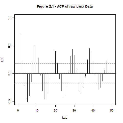
5acf(dat, 50, main = "Figure 2.1 - ACF of raw Lynx Data")
1pacf(dat, 50, main = "Figure 2.2 - PACF of raw Lynx Data")

To achieve stationary residuals the seasonality of the data was investigated. Examining the ACF seemed to indicate a 10 year seasonal trend (Fig 2), however differencing the data did not improve the oscillations present in the ACF. It seems that the peaks, despite their apparent periodicity, are not predictable. Because of this we will not make any models that had a seasonal component.
Looking at the variance
Lets look at the variance for the first half of the dataset, and the second half.
 1data = dat
 2first = data[1:(length(data)/2)]
 3second = data[(length(data)/2+1): (length(data))]
 4
 5var(first)
 6
 7## [1] 2316637
 8
 9mean(first)
10
11## [1] 1458.158
12
13var(second)
14
15## [1] 2745091
16
17mean(second)
18
19## [1] 1617.877
The second half has slightly more variance.
##Lets transform the data to depress this variance. We can log the data to depress the variance a bit
1d.log = log(dat)
2plot(d.log)
![]()
 1data = d.log
 2first = data[1:(length(data)/2)]
 3second = data[(length(data)/2+1): (length(data))]
 4
 5var(first)
 6
 7## [1] 1.382848
 8
 9mean(first)
10
11## [1] 6.703306
12
13var(second)
14
15## [1] 1.952537
16
17mean(second)
18
19## [1] 6.66856
20
21var(first) - var(second)
22
23## [1] -0.569689
24
25hist(dat, main = "Figure 3 - untransformed Lynx data")
![]()
1hist(d.log, main = "Figure 4 - transformed Lynx data")
![]()
The log transformed is MUCH better.
Trying to "detrend"
1trend =
2d.log.detrend <- resid(lm(d.log ~ time(d.log)))
3
4plot(d.log.detrend, type = "l", main = "Figure 5 - detrended and log transformed Lynx data")

1hist(d.log.detrend)

1#this looks pretty good now.
We can also attempt to remove a seasonal component to the data. Below is the code for that, but we won't run it because it doesn't improve stationarity. So, despite what it appears to be, once log transformed and detrended the lynx data is already stationary!
Removing seasonal trends - how you would do it, though it doesn't work for this dataset.
 1#the pacf component appears to be an AR(2)
 2#attempt at removing a "seasonal" component - to no avail.
 3d.log
 4for(i in c(1:10)){
 5plot(diff(dat, lag = i))
 6}
 7
 8#differencing makes almost no difference.
 9#none of the plots look improved.
10#It seems that the peaks, despite their apparent periodicity, are not predictable.
Choose a model to fit the residuals.
Lets test som models on this data. We are fitting "ARIMA" models, or Auto Regressive Integrated Moving Average models. These models have three components, p, d, and q. The parameters of the ARIMA model are defined as follows:
p: The number of lag observations included in the model, also called the lag order. d: The number of times that the raw observations are differenced, also called the degree of differencing. q: The size of the moving average window, also called the order of moving average.
The syntax for ARIMA models is generally Arima(p,d,q). So in the example below, we are comparing a ARIMA(2,0,1) and an ARIMA(2,0,2).
1#lets test some models on this data.
2
3acf.d = acf2(d.log.detrend, 50)

 1mod.1 = sarima(d.log.detrend, 2,0,1)
 2
 3## initial  value 0.249436
 4## iter   2 value -0.309862
 5## iter   3 value -0.370696
 6## iter   4 value -0.477115
 7## iter   5 value -0.509287
 8## iter   6 value -0.534067
 9## iter   7 value -0.571560
10## iter   8 value -0.595904
11## iter   9 value -0.621684
12## iter  10 value -0.651739
13## iter  11 value -0.652590
14## iter  12 value -0.657683
15## iter  13 value -0.660312
16## iter  14 value -0.661080
17## iter  15 value -0.661131
18## iter  16 value -0.661132
19## iter  17 value -0.661132
20## iter  17 value -0.661132
21## iter  17 value -0.661132
22## final  value -0.661132
23## converged
24## initial  value -0.655726
25## iter   2 value -0.655820
26## iter   3 value -0.655844
27## iter   4 value -0.655875
28## iter   5 value -0.655891
29## iter   6 value -0.655894
30## iter   7 value -0.655895
31## iter   7 value -0.655895
32## iter   7 value -0.655895
33## final  value -0.655895
34## converged

 1mod.2 = sarima(d.log.detrend, 2,0,2)
 2
 3## initial  value 0.249436
 4## iter   2 value -0.320525
 5## iter   3 value -0.442471
 6## iter   4 value -0.498334
 7## iter   5 value -0.516408
 8## iter   6 value -0.526464
 9## iter   7 value -0.530492
10## iter   8 value -0.536595
11## iter   9 value -0.601440
12## iter  10 value -0.609549
13## iter  11 value -0.640524
14## iter  12 value -0.652371
15## iter  13 value -0.658401
16## iter  14 value -0.658846
17## iter  15 value -0.660549
18## iter  16 value -0.664565
19## iter  17 value -0.664603
20## iter  18 value -0.664611
21## iter  19 value -0.664614
22## iter  20 value -0.664614
23## iter  20 value -0.664614
24## iter  20 value -0.664614
25## final  value -0.664614
26## converged
27## initial  value -0.659301
28## iter   2 value -0.659396
29## iter   3 value -0.659422
30## iter   4 value -0.659452
31## iter   5 value -0.659462
32## iter   6 value -0.659466
33## iter   7 value -0.659467
34## iter   8 value -0.659468
35## iter   8 value -0.659468
36## iter   8 value -0.659468
37## final  value -0.659468
38## converged

1mod.1$AICc
2
3## [1] -0.2421902
4
5mod.2$AICc
6
7## [1] -0.2299404
Based on the ACF and PACF of the now stationary series, the better model from our two models is an ARIMA(2,0,1) model (Fig. 6). From the ACF we see that it is most likely MA(1), though MA(2) is also a possibility. From the PACF we can see that it is AR(2) due to the two strong peaks.
What is the model obtained by using AICC? Is it same as one of the models suggested by ACF/PACF?
We can compare a number of models this way. We will not run this code because it takes up lots of space, but feel free to run and observe on your own.
 1#generating models with p and q values of either 0, 1, or 2.
 2
 3P <-0
 4S <- 0
 5Q <- 0
 6bic.m <- matrix(c(rep(NA,9)),3,3)
 7aic.m <- matrix(c(rep(NA,9)),3,3)
 8logL.m <- matrix(c(rep(NA,9)),3,3)
 9for (p in c(0,1,2))
10  for(q in c(0,1,2))
11  {
12    smod <- sarima(d.log.detrend, p, 0, q, 0, 0, 0, 0) # fit model
13    bic.m[p+1,q+1] <- smod$BIC
14    aic.m[p+1,q+1] <- smod$AICc
15    logL.m[p+1,q+1] <- -smod$fit$loglik
16  }
17
18bic.m
19aic.m
To examine other models besides the one selected based off of the ACF and PACF plots, models were generated used for-loops and then compared using BIC and AICc values (Tables 1, 2). The BIC matrix shows that the model supported by the BIC values (i.e. the lowest matrix value) is an ARMA(2, 0, 0) with a BIC value of -1.1857. This is almost indistinguishable from the next lowest model, an ARMA(2,0,1), which is the model supported by my model choice based off of the ACF and PACF, BIC value of -1.1686. When looking at the AICc values the lowest value is an ARMA(2,0,2) model, however the AICc values are all essentially the same. In fact, none of the values are far enough apart to merit real distinction between models.
Estimate the parameters of the model and write down the model in algebraic form.
 1#turning model into an arima() model to get the coef. and variance estimates
 2
 3mod.1.1 = arima(d.log.detrend, c(2,0,1))
 4
 5#The equation for this model is
 6
 7mod.1.1$coef
 8
 9##          ar1          ar2          ma1    intercept
10##  1.475280551 -0.816861229 -0.233232740 -0.001533242
11
12    #Xt = 1.47531*Xt-1 + -0.8169*Xt-2 + -0.2332*Wt-1 + Wt
13
14#(d) What is the variance estimate?
15
16var = mod.1.1$var.coef
17var
18
19##                     ar1           ar2           ma1     intercept
20## ar1        4.760036e-03 -3.607999e-03 -0.0055806041 -6.405797e-05
21## ar2       -3.607999e-03  3.689721e-03  0.0039856618  6.112233e-05
22## ma1       -5.580604e-03  3.985662e-03  0.0150024841  1.373257e-04
23## intercept -6.405797e-05  6.112233e-05  0.0001373257  1.179494e-02
Because the models are essentially identical, we'll am going with the initial model choice of an ARMA(2,0,1). This model can be written as
X_t=1.4753X_(t-1)+ -0.8169X_(t-2)+ -0.2332W_(t-1)
We estimated the parameters using the Maximum Likelihood Method (which is the default in both arima() and sarima()). We used this used that estimate method because the MLE method is preferred for ARMA(p,q) models and this model was an ARMA(2,1) (Shumway and Stoffer pg. 78) .
The variance in the estimates was produced using the arima() command as well, and can be seen above.
Do the diagnostic checking, plot the residuals of the fitted model.
1#Plot the autocorrelations of the residuals. Are their any outliers?
2
3resid = mod.1.1$residuals
4
5plot(resid, main = "Figure 7 - Plot of Residuals")

1acf(resid, 1000)

1  #the plot of the residuals seems to show that, although very spiky, there are not any dramatic outliers.
2  #the acf plot shows that this could be improved a bit, but we already knew that since the model is relatively poor. :/
3
4#Perform tests (chi-squared, and so on) of randomness and obtain the p-values.
5
6resid.nom = as.numeric(mod.1.1$residuals[1:114])
7hist(resid.nom, main = "Figure 8 - Histogram of Residuals")

 1#pretty dang normal
 2
 3#to test for the randomness I am using a Kolmogorov-Smirnov test.
 4#This test is like the chi squared test in that it compares my distribution to an expected distributin (in this case rnorm)
 5#but this test can also take continuous vectors
 6
 7randomness.test = ks.test(resid.nom, rnorm(
 8  n = length(resid.nom),
 9  mean = mean(resid.nom),
10  sd = sd(resid.nom))
11  )
12
13randomness.test$p.value
14
15## [1] 0.6634279
16
17#the p-value shows that the residuals are essentially random
We ran model diagnostics by looking at a plot of the residuals, a histogram of the residuals, and performing a Kolmogorov-Smirnov test. The Kolmogorov-Smirnov test is like the Chi Squared test in that it compares the distribution to an expected distributing (in this case rnorm) but this test can also take continuous vectors. We also investigated the Ljung-Box plot provided by the sarima() function, and a long term ACF of the residuals.
From the residuals we can conclude that the model is satisfactory, though not optimum. By looking at the Ljung-Box values shows that at higher lags they are below the interval (i.e. not independent) yet looking at a long term ACF of the residuals shows that the longer lags are not having an impact. The plot of the residuals, although very spiky, showed no dramatic outliers and the histogram was relatively normal, Figures 7 and 8 respectively. The Kolmogrorov-Smirnov test showed that the residuals were essentially random (p-value = 0.7727)). Based on the Kolmogorov-Smirnov test, and the histogram of the residuals, the model is ok.
Forecast the last 10 values based on our one chosen model.
1#Plot the original series and the forecasts for both of them.
2
3short = d.log.detrend[1:(length(d.log.detrend)-10)]
4
5forcasted = sarima.for(short, p = 2, d = 0, q = 1, n.ahead = 10)

 1forcasted$pred
 2
 3## Time Series:
 4## Start = 105
 5## End = 114
 6## Frequency = 1
 7##  [1]  1.25441563  1.03999995  0.50228428 -0.11783032 -0.59539761
 8##  [6] -0.79468001 -0.69886516 -0.39410970 -0.02162615  0.28014816
 9
10#Now lets calculate the 95% confidence intervals for the prediction values.
11
12lower = forcasted$pred-1.96*forcasted$se
13upper = forcasted$pred+1.96*forcasted$se
14
15lower
16
17## Time Series:
18## Start = 105
19## End = 114
20## Frequency = 1
21##  [1]  0.2150928 -0.6093246 -1.4499465 -2.1324971 -2.6135223 -2.8949890
22##  [7] -2.9338470 -2.7229627 -2.3756480 -2.0740342
23
24upper
25
26## Time Series:
27## Start = 105
28## End = 114
29## Frequency = 1
30##  [1] 2.293738 2.689325 2.454515 1.896836 1.422727 1.305629 1.536117
31##  [8] 1.934743 2.332396 2.634331
32
33#Plotting it all together
34plot(d.log.detrend, type = "l", main = "Figure 9 - Real Lynx data and Forecasted Values")
35
36lines(forcasted$pred, type = "p", col = "red", lwd = 2)
37#adding confidence intervals
38lines(upper, type = "l", lty=2, lwd=1, col = "blue")
39lines(lower, type = "l", lty=2, lwd=1, col = "blue")
