Mapping in R

Apr 30, 2018 · 10 min read · cowplot grid mapping mapview sf spatial data spData spDataLarge tidyverse tmap ·

Post by Dominik Schneider

A couple things to note. Spatial/gis functions in R are undergoing a massive change right now. The old stalwart sp has been succeeded by sf (simple features), which is compatible with the open geospatial consortium standards. When you are looking for solutions online, make sure you know which data type is being used- they are not interchangeable. You can convert from sf to sp with as(x,'Spatial') and vice versa with st_as_sf(). Stick with sf whenever possible, it is the future. sf is designed to be more consistent in syntax, tidy, and feature rich (it does everything rgdal, rgeos, and sp do/did).

sf is specific to vector data (points, lines, polygons). Gridded raster data is still served by raster. Unfortunately, thye are not really compatible so if you need to mix them, you will need to convert your sf objects to sp objects. This should mostly only be the case for analysis because there are mapping packages that handle both. Keep your eye on star as an upcoming successor of the raster package.

If you do need to mix vector and raster data, I think it's still worth doing any vector operations with sf and then convert to sp at the end. I believe many of the sf tools are written in c++ to be as efficient as possible. For polygon/raster conversions, check out fasterize and spex for more efficient implementations that work with sf. I often just convert my raster and vector data to tibbles and use the tidyverse tools to do the processing.

If there is one resource you should read, it's the new Geocomputation with R book that is being written. Basic spatial methods are described in part 1 and I will assume some knowledge of that material. I am going to cover mapping from part 2.

They recommend tmap because it can handle sp, sf, and raster objects. You will see it's quite powerful. I encourage you to read the vignettes.

load libraries

 1# these packages can be installed from cran
 2require(sf) # the spatial workhorse
 3
 4## Loading required package: sf
 5
 6## Warning: package 'sf' was built under R version 3.4.4
 7
 8## Linking to GEOS 3.6.1, GDAL 2.2.3, proj.4 4.9.3
 9
10library(spData) #example spatial data
11
12## Warning: package 'spData' was built under R version 3.4.4
13
14library(tidyverse) # for general data wrangling
15
16## -- Attaching packages ---------------------------------- tidyverse 1.2.1 --
17
18## v ggplot2 2.2.1.9000     v purrr   0.2.4
19## v tibble  1.4.2          v dplyr   0.7.4
20## v tidyr   0.8.0          v stringr 1.3.0
21## v readr   1.1.1          v forcats 0.3.0
22
23## Warning: package 'tidyr' was built under R version 3.4.4
24
25## Warning: package 'stringr' was built under R version 3.4.4
26
27## Warning: package 'forcats' was built under R version 3.4.4
28
29## -- Conflicts ------------------------------------- tidyverse_conflicts() --
30## x dplyr::filter() masks stats::filter()
31## x dplyr::lag()    masks stats::lag()
32
33library(tmap)    # for static and interactive maps
34library(mapview) # for interactive maps
35
36## Warning: package 'mapview' was built under R version 3.4.4
37
38library(grid) # for putting multiple plot on top of each other
39library(cowplot) # for arranging multiple ggplots
40
41##
42## Attaching package: 'cowplot'
43
44## The following object is masked from 'package:ggplot2':
45##
46##     ggsave
47
48# install with install.packages("spDataLarge", repos = "https://nowosad.github.io/drat/", type = "source")
49library(spDataLarge) # more example spatial data

the data

I will use the new zealand example dataset from spData, but if you need to read in your own GIS data you can use the built in functions from sf::read_sf() for vector data and raster::raster() for raster data.

If you have a csv file with coordinates for points try this general approach:

csvdata <- readr::read_csv(file=<your_filename>)
sfdata <- sf::st_as_sf(csvdata,
                       coords = c('xcoords','ycoords'),
                       crs = <a_proj4_projection_string>)

Example datasets in spData include nz. It is a multipolygon simple feature collection of New Zealand.

 1spData::nz
 2
 3## Simple feature collection with 16 features and 6 fields
 4## geometry type:  MULTIPOLYGON
 5## dimension:      XY
 6## bbox:           xmin: 1090144 ymin: 4748537 xmax: 2089533 ymax: 6191874
 7## epsg (SRID):    2193
 8## proj4string:    +proj=tmerc +lat_0=0 +lon_0=173 +k=0.9996 +x_0=1600000 +y_0=10000000 +ellps=GRS80 +towgs84=0,0,0,0,0,0,0 +units=m +no_defs
 9## First 10 features:
10##    REGC2017            REGC2017_NAME AREA_SQ_KM LAND_AREA_SQ_KM
11## 1        01         Northland Region  12512.749       12500.320
12## 2        02          Auckland Region   4942.693        4941.622
13## 3        03           Waikato Region  24578.246       23899.899
14## 4        04     Bay of Plenty Region  12280.444       12070.497
15## 5        05          Gisborne Region   8385.816        8385.816
16## 6        06       Hawke's Bay Region  14191.302       14137.210
17## 7        07          Taranaki Region   7254.357        7254.357
18## 8        08 Manawatu-Wanganui Region  22220.590       22220.590
19## 9        09        Wellington Region   8119.553        8048.661
20## 10       12        West Coast Region  23319.648       23243.812
21##    Shape_Length  Shape_Area                       geometry
22## 1     3321236.6 12512734660 MULTIPOLYGON (((1745493 600...
23## 2     2878758.5  4942685973 MULTIPOLYGON (((1793982 593...
24## 3     2177078.9 24578239227 MULTIPOLYGON (((1860345 585...
25## 4     1400381.0 12280442951 MULTIPOLYGON (((2049387 583...
26## 5      689546.8  8385816413 MULTIPOLYGON (((2024489 567...
27## 6      948804.8 14191296978 MULTIPOLYGON (((2024489 567...
28## 7      533923.9  7254385835 MULTIPOLYGON (((1740438 571...
29## 8     1118235.5 22220599731 MULTIPOLYGON (((1866732 566...
30## 9      679244.2  8119550321 MULTIPOLYGON (((1881590 548...
31## 10    1723903.1 23319649647 MULTIPOLYGON (((1557042 531...

simple examples

The basic tmap syntax includes a spatial object in tm_shape plus a layer that you choose based on the geometry you are trying to plot. You can add multiple layers for a given object.

1tm_shape(nz) + tm_fill()

1# Add border layer to nz shape
2tm_shape(nz) + tm_borders()

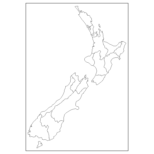
1# Add fill and border layers to nz shape
2tm_shape(nz) + tm_fill() + tm_borders()

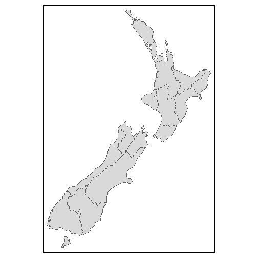
tmap uses the "grammar of graphics" similar to ggplot. You can create maps by adding layers on top of each other.

1map_nz = tm_shape(nz) + tm_polygons() #tm_polygons is the equivalent to tm_fill+tm_borders
2
3map_nz + # note that you can store maps as objects
4  tm_shape(nz_elev) + tm_raster(alpha = 0.7)

Data-defined plotting

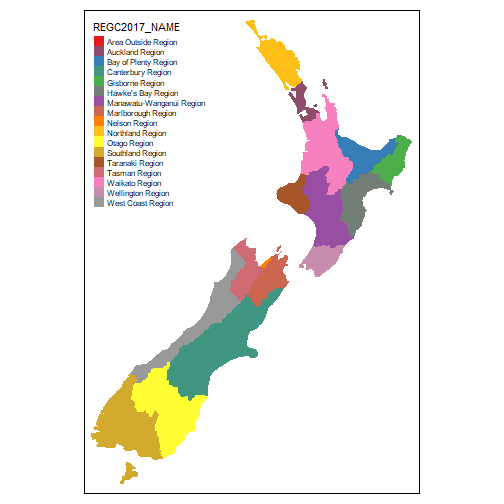
It's also simple to color your features by a variable.

1tm_shape(nz)+tm_fill(col='REGC2017_NAME')

Want to change the colors? check out the nifty tmaptools::palette_explorer()

1tm_shape(nz)+tm_fill(col='REGC2017_NAME', palette='Set1')

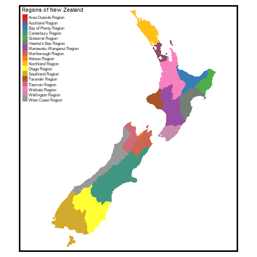
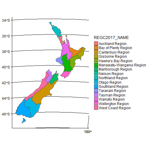
You can use tm_layout to adjust layout options, like margins. Here is an example where I made more space for the legend.

 1tm_shape(nz)+
 2  tm_fill(col='REGC2017_NAME',
 3          palette='Set1',
 4          title='Regions of New Zealand')+
 5  tm_layout(frame.lwd = 5,
 6            legend.just = c(0,1),
 7            legend.position = c(0.01,1),
 8            inner.margins = c(.02,.15,0.02,.1),
 9            legend.width = 0.5)+
10  tm_style_beaver()

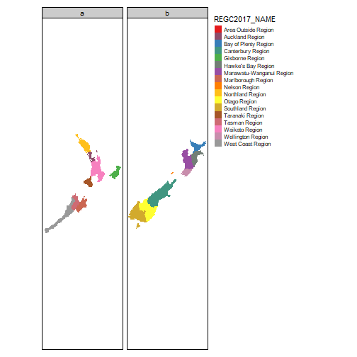
Facetting based on data categories

If you have data, for example for different months or years, you could plot them simulataneously with a shared legend.

1# make a random category
2nz$let=sample(letters[1:2],nrow(nz),replace=T)
3
4# here is a silly map based on randomly assigned 'a' or 'b'
5tm_shape(nz)+
6  tm_fill(col='REGC2017_NAME', palette='Set1')+
7  tm_facets(by='let')

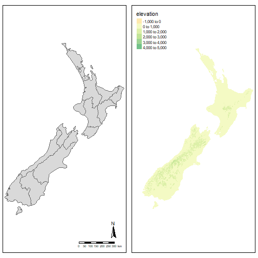
Arrange different types of plots next to each other

If you have two (or more) maps you would like side by side that you can't split based on an attribute you might find it useful to use tmap_arrange. You can also easily add a north arrow and scalebar.

1tmap_arrange(map_nz + tm_compass() + tm_scale_bar() ,
2             tm_shape(nz_elev) + tm_raster(alpha = 0.7),
3             ncol=2)

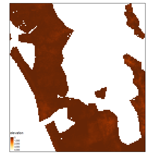
inset maps

 1# compute the bounding box for the auckland region
 2auckland_box <- st_bbox(nz %>% filter(REGC2017_NAME=='Auckland Region')) %>%
 3  st_as_sfc()
 4
 5## Warning: package 'bindrcpp' was built under R version 3.4.4
 6
 7# create a map of elevation for the subset we want to blow up
 8auckland_elev <-
 9  tm_shape(spDataLarge::nz_elev,
10           ylim=c(5871375, 6007878),
11           xlim=c(1704673,1828993))+
12  tm_raster(style = "cont", palette='-YlOrBr',#minus sign for the palette reverses the colors
13            auto.palette.mapping = FALSE, legend.show = TRUE)+
14  tm_legend(legend.just=c(0,0),
15            legend.position=c(0,0))
16auckland_elev

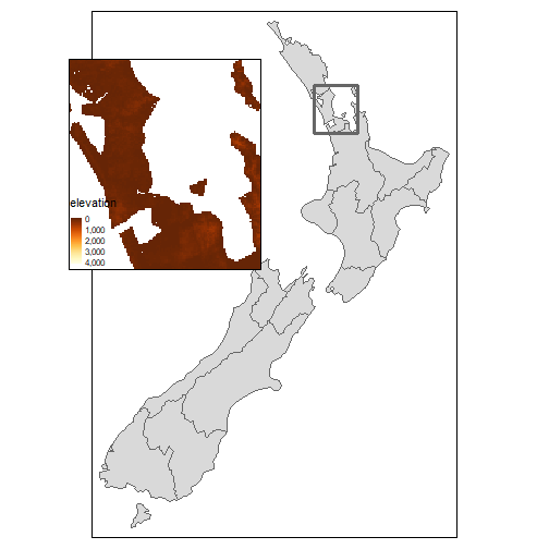
1# make the overview map tha tincludes a box outlining our subset we are highlighting
2bigmap <- map_nz +
3  tm_shape(auckland_box) +  #here we are adding the little inset box on the overview map
4  tm_borders(lwd = 3)
5bigmap

1# make a viewport. think of this as a window in the bigmap through whcih we can see the elevation inset
2auckland_vp <- grid::viewport(0.3, 0.7, width = 0.4, height = 0.4)
3
4#make sure you run these next lines all at once to see the result!
5bigmap
6print(auckland_elev, vp = auckland_vp)

 1# save your map using standard graphic functions - pdf()...dev.off() or save_tmap()
 2save_tmap(tm=bigmap,
 3          filename='test_map.png',
 4          insets_tm=auckland_elev,
 5          insets_vp=auckland_vp)
 6
 7## Map saved to D:\Labou\Misc\R_working_group\test_map.png
 8
 9## Resolution: 2100 by 2100 pixels
10
11## Size: 6.999999 by 6.999999 inches (300 dpi)

interactive maps!

See the tmap vignette or the mapview vignettes. mapview probably has more interactive features and supports more object types.

for ggplot purists

If you don't know ggplot already, stick with tmap to begin with. if you are a ggplot enthusiast, you should know that the development version of ggplot has a new geom - geom_sf - that will make map making easier and more robust!

you can install the development ggplot with:

1# geom_sf still in ggplot dev. will need to install devtools from cran first
2install.packages('devtools')
3devtools::install_github("tidyverse/ggplot2")
4library(ggplot2)

simple example with geom_sf

1ggplot()+
2  geom_sf(data=nz,aes(fill=REGC2017_NAME))+
3  coord_sf() #handles projections!

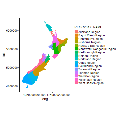
the old way

what a mess, especially if you want the data and spatial info in your dataframe! for more, see the CU Earth Lab tutorial

 1# polygons require a trip through 'sp', and then a join to get your data back
 2nz.sp <- as(nz,'Spatial')
 3
 4nz.df <- broom::tidy(nz.sp,region='REGC2017') %>%
 5  full_join(nz.sp@data ,by=c('id'='REGC2017'))
 6
 7## Warning: Column `id`/`REGC2017` joining character vector and factor,
 8## coercing into character vector
 9
10ggplot()+
11  geom_polygon(data=nz.df,aes(x=long,y=lat,group=group,fill=REGC2017_NAME))+
12  coord_fixed(ratio = 1) #you need to make sure things are in the right projection

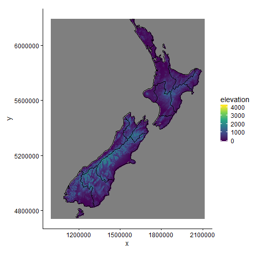
1nz_elev_df <- raster::as.data.frame(nz_elev,xy=T)
2
3ggplot()+
4  geom_raster(data=nz_elev_df,aes(x=x,y=y,fill=elevation))+
5  scale_fill_viridis_c()+
6  geom_path(data=nz.df,aes(x=long,y=lat,group=group))+
7  coord_fixed(ratio=1)

1# normally you can use ggsn package to add north arrow and scale bar but it's not working well right now, maybe because I'm using the dev ggplot

inset maps and multiple plots side by side - cowplot

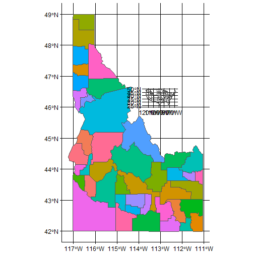
If you use ggplot, you need to learn cowplot. Your life will be exponentially improved. We can use the cowplot package to place multiple ggplot figures next to each other or within each other.

Here is a basic example of cowplot's capabilities. Obviously the formatting and legend need some work, but hopefully you get the idea!

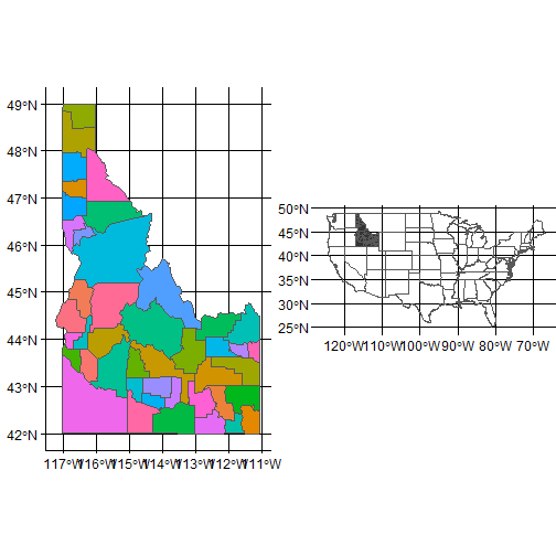
 1# get some data from maps
 2usa <- st_as_sf(maps::map('state',plot=F, fill=T))
 3counties <- sf::st_as_sf(maps::map(database='county',regions='idaho',fill=TRUE,plot=F))
 4
 5# plot the counties of Idaho
 6gidaho <-
 7  ggplot(counties)+
 8  geom_sf(aes(fill=ID),show.legend = F)
 9# gidaho
10
11# create a ggplot of usa
12overview <-
13  ggplot(usa)+
14  geom_sf(fill=NA)+
15  geom_sf(data=counties,fill='grey20')+
16  # blank()+
17  theme(axis.line=element_blank(),
18        plot.margin= unit(c(0,0,0,0),'npc'))
19# overview
20
21# combine the two ggplot objects, with the overview map of the usa as an inset
22cowplot::ggdraw(gidaho)+
23  cowplot::draw_plot(overview,0.5,0.5,.2,.2,scale=1)

1# combine the two ggplot objects by placing them side by side
2cowplot::plot_grid(gidaho,overview)

Miscellaneous

There are many other ways to create maps in R, but I recommend becoming proficient in 1 rather than jumping around.

The one other exciting tool is ggmap - which will download background maps from google maps, stamen, open street map. This does not work easily with tmap. Theoretically it works well with ggplot but there are still some issues to be worked out with the new dev version.

If you want to give ggmap a go with the pre-geom_sf ggplot (v2.2.1), check out this tutorial.

tmap can currently only download background maps in interactive "view" mode (v2 will support basemaps in "plot" mode, which you can try out by installing the development version directly from github). dismo::gmap and Rgooglmaps may provide options for static plots on background maps.

If you are using interactive maps, check out these (background maps)[https://leaflet-extras.github.io/leaflet-providers/preview/] that you can use with tmap in view mode.

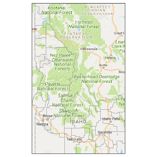
quick example with `dismo::gmap` and `tmap`

 1# dismo::gmap returns a raster with projection string so you can use it with tmap
 2library(dismo)
 3
 4## Warning: package 'dismo' was built under R version 3.4.4
 5
 6## Loading required package: raster
 7
 8## Loading required package: sp
 9
10## Warning: package 'sp' was built under R version 3.4.4
11
12##
13## Attaching package: 'raster'
14
15## The following object is masked from 'package:dplyr':
16##
17##     select
18
19## The following object is masked from 'package:tidyr':
20##
21##     extract
22
23## The following object is masked from 'package:ggplot2':
24##
25##     calc
26
27id2 <- dismo::gmap('idaho',type='roadmap',lonlat = T)
28
29# use the builtin maps package to download counties of Idaho
30counties <- sf::st_as_sf(maps::map(database='county',regions='idaho',fill=TRUE,plot=F))
31
32tmap_mode('plot')
33
34## tmap mode set to plotting
35
36tm_shape(id2,
37         bbox = tmaptools::bb(counties))+
38  tm_raster()+
39  tm_shape(counties)+
40  tm_borders(alpha=0.5)