Nonlinear regression tutorial

 1#simulate some data
 2#set random number generator
 3set.seed(2019)
 4x<-seq(0,50,1)
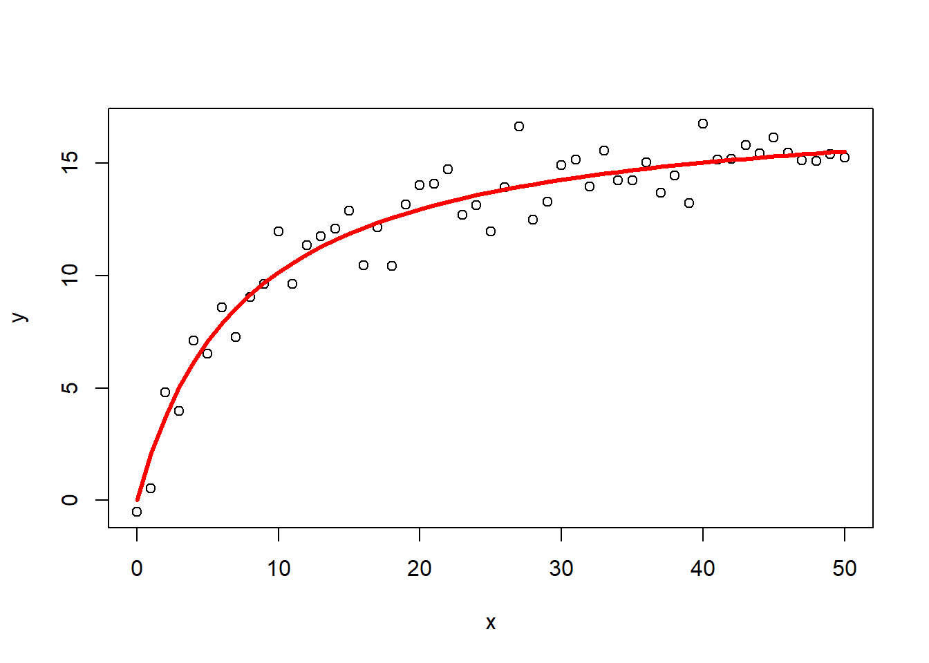
 5y<-((runif(1,10,20)*x)/(runif(1,0,10)+x))+rnorm(51,0,1)
 6#for simple models nls find good starting values for the parameters even if it throws a warning
 7
 8#Michaelis-Menten equation
 9m<-nls(y~a*x/(b+x))
10
11## Warning in nls(y ~ a * x/(b + x)): No starting values specified for some parameters.
12## Initializing 'a', 'b' to '1.'.
13## Consider specifying 'start' or using a selfStart model
14
15m
16
17## Nonlinear regression model
18##   model: y ~ a * x/(b + x)
19##    data: parent.frame()
20##      a      b
21## 17.908  7.645
22##  residual sum-of-squares: 51.78
23##
24## Number of iterations to convergence: 6
25## Achieved convergence tolerance: 1.077e-06
26
27#will throw warning, but should work
28#get some estimation of goodness of fit
29cor(y,predict(m))
30
31## [1] 0.9658715
32
33#plot
34plot(x,y)
35lines(x,predict(m),col="red",lwd=3)

 1#simulate some data, this without a priori knowledge of the parameter value
 2x<-seq(0,50,1)
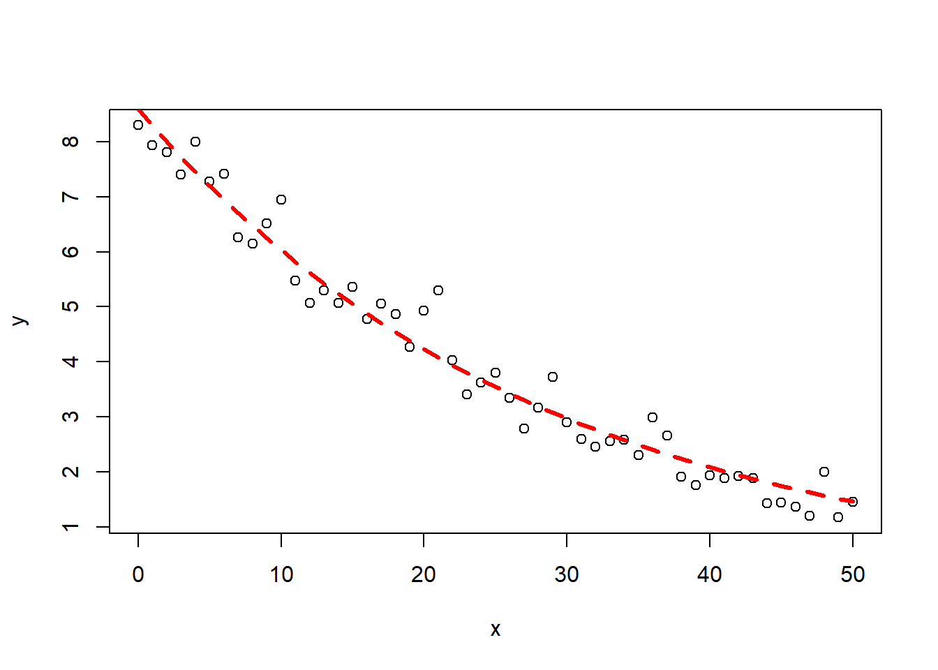
 3y<-runif(1,5,15)*exp(-runif(1,0.01,0.05)*x)+rnorm(51,0,0.5)
 4#visually estimate some starting parameter values
 5plot(x,y)
 6
 7#from this graph set approximate starting values
 8a_start<-8 #param a is the y value when x=0
 9b_start<-log(0.1)/(50*8) #b is the decay rate. k=log(A)/(A(intial)*t)
10
11#model
12m1<-nls(y~a*exp(-b*x),start=list(a=a_start,b=b_start))
13m1
14
15## Nonlinear regression model
16##   model: y ~ a * exp(-b * x)
17##    data: parent.frame()
18##       a       b
19## 8.59328 0.03544
20##  residual sum-of-squares: 7.588
21##
22## Number of iterations to convergence: 6
23## Achieved convergence tolerance: 7.615e-07
24
25#get some estimation of goodness of fit (should be closer to 1)
26cor(y,predict(m1))
27
28## [1] 0.9833285
29
30#plot the fit
31lines(x,predict(m1),col="red",lty=2,lwd=3)

 1library(deSolve) #this package is good for solving differential equations
 2#simulating some population growth from the logistic equation and estimating the parameters using nls
 3
 4#defining a function
 5log_growth <- function(Time, State, Pars) {
 6  with(as.list(c(State, Pars)), {
 7    dN <- R*N*(1-N/K)
 8    return(list(c(dN)))
 9  })
10}
11#Time is the time intervals, States are the variable names, Pars and parameters
12
13#pars, N_int, tmes are used to simulate data
14pars  <- c(R=0.2,K=1000) #the parameters for the logisitc growth
15N_ini <- c(N=1) #the initial numbers
16times <- seq(0, 50, by = 1) #the time step to evaluate
17
18#the ODE (ordinary differential equation)
19out <- ode(N_ini, times, log_growth, pars)
20plot(out)

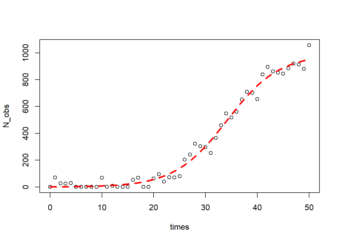
 1#add some random variation to it
 2N_obs<-out[,2]+rnorm(51,0,50)
 3#remove numbers less than 1
 4N_obs<-ifelse(N_obs<1,1,N_obs)
 5#plot
 6plot(times,N_obs)
 7
 8#Not having starting values only works sometimes with simple data and functions like in the first example.
 9#notice how m3 WON'T work.Remember nls iteritavely runs to converge and this will not converge in under 30 iterations
10#m3<-nls(N_obs~K*N0*exp(R*times)/(K+N0*(exp(R*times)-1)))
11
12#getInitial gives guesses on parameter values based on data
13#SSlogis is a selfStarting model
14SS<-getInitial(N_obs~SSlogis(times,alpha,xmid,scale),data=data.frame(N_obs=N_obs,times=times))
15#follows this equation: N(t)=alpha/(1+e+((xmid-t)/scale)
16SS
17
18##      alpha       xmid      scale
19## 991.798725  34.112932   5.045119
20
21#need to do some algebra to get parameterization right
22#we used a different parametrization
23K_start<-SS["alpha"]
24R_start<-1/SS["scale"]
25N0_start<-SS["alpha"]/(exp(SS["xmid"]/SS["scale"])+1)
26#the formula (not set up as differential equation) for the model
27log_formula<-formula(N_obs~K*N0*exp(R*times)/(K+N0*(exp(R*times)-1)))
28
29#fit the model
30m4<-nls(log_formula,start=list(K=K_start,R=R_start,N0=N0_start))
31
32#estimated parameters
33summary(m4)
34
35##
36## Formula: N_obs ~ K * N0 * exp(R * times)/(K + N0 * (exp(R * times) - 1))
37##
38## Parameters:
39##           Estimate Std. Error t value Pr(>|t|)
40## K.alpha  991.79872   29.86851  33.205   <2e-16 ***
41## R.scale    0.19821    0.01338  14.817   <2e-16 ***
42## N0.alpha   1.14659    0.47931   2.392   0.0207 *
43## ---
44## Signif. codes:  0 '***' 0.001 '**' 0.01 '*' 0.05 '.' 0.1 ' ' 1
45##
46## Residual standard error: 44.08 on 48 degrees of freedom
47##
48## Number of iterations to convergence: 0
49## Achieved convergence tolerance: 4.177e-06
50
51#get some estimation of goodness of fit (should be closer to 1)
52cor(N_obs,predict(m4))
53
54## [1] 0.9925536
55
56#plot
57lines(times,predict(m4),col="red",lty=2,lwd=3)

1library(growthrates)
2
3time<-rep(1:25, 8)
4y<-grow_logistic(time, c(y0=0.2, mumax=0.3, K=4))[,"y"]
5y<-jitter(y, factor=1, amount=0.3)
6data<-data.frame(cbind(time,y))
7data<-data[order(data$y),]
8data$ID<-c(rep(1:10,20))
9plot(time,y)

 1splitted.data <- multisplit(data, c("ID"))
 2
 3## show which experiments are in splitted.data
 4names(splitted.data)
 5
 6##  [1] "1"  "2"  "3"  "4"  "5"  "6"  "7"  "8"  "9"  "10"
 7
 8## get table from single individual.  Or could be an experiment, or batch, or block, etc.
 9dat <- splitted.data[["1"]]
10dat[1, 2] = 0.03
11
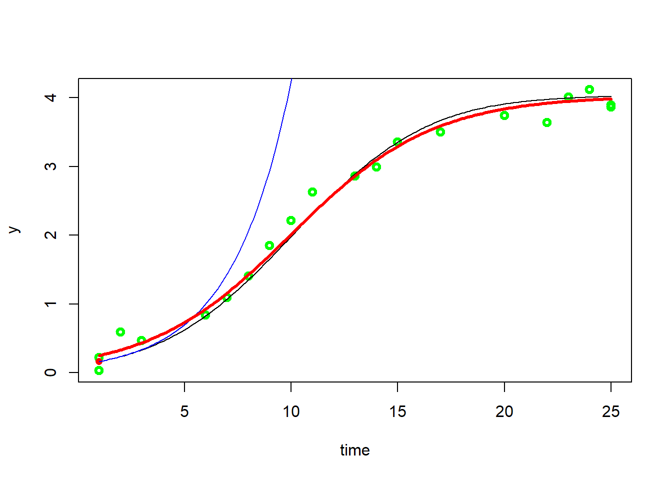
12fit0 <- fit_spline(dat$time, dat$y)
13plot(fit0, col="green", lwd=3)
14summary(fit0)
15
16## Fitted smoothing spline:
17## Call:
18## smooth.spline(x = time, y = ylog)
19##
20## Smoothing Parameter  spar= 0.6721364  lambda= 0.006882113 (12 iterations)
21## Equivalent Degrees of Freedom (Df): 3.685259
22## Penalized Criterion (RSS): 2.029662
23## GCV: 0.3015
24##
25## Parameter values of exponential growth curve:
26## Maximum growth at x= 1.001382 , y= 0.1644875
27## y0 = 0.1145593
28## mumax = 0.3612431
29##
30## r2 of log transformed data= 0.8652797
31
32#can get maximum growth rate from here.  Plot will show the exponetial curve (blue line) from max rate
33
34## initial parameters
35p <- c(coef(fit0), K = max(dat$y))
36
37## avoid negative parameters
38lower = c(y0 = 0, mumax = 0, K = 0)
39
40fit3<-fit_growthmodel(grow_logistic, p=p, time=data$time, y=data$y)
41lines(fit3, col="red", lwd=3)

 1summary(fit3)
 2
 3##
 4## Parameters:
 5##       Estimate Std. Error t value Pr(>|t|)
 6## y0    0.188670   0.012562   15.02   <2e-16 ***
 7## mumax 0.301080   0.007458   40.37   <2e-16 ***
 8## K     4.027982   0.029659  135.81   <2e-16 ***
 9## ---
10## Signif. codes:  0 '***' 0.001 '**' 0.01 '*' 0.05 '.' 0.1 ' ' 1
11##
12## Residual standard error: 0.1713 on 197 degrees of freedom
13##
14## Parameter correlation:
15##            y0   mumax       K
16## y0     1.0000 -0.9448  0.5116
17## mumax -0.9448  1.0000 -0.6615
18## K      0.5116 -0.6615  1.0000
19
20#Get parameters for the entire population
21
22fit4<-all_growthmodels(
23          y ~ grow_logistic(time, parms) | ID,
24          data = data, p = p, lower = lower) #gives parameters for each individual
25
26results(fit4, extended=TRUE) #extended gives you time estimates of saturation values.
27
28##    ID        y0     mumax        K turnpoint     sat1     sat2     sat3
29## 1   1 0.1775788 0.3186817 3.922830  9.567004 13.69952 15.84286 18.80644
30## 2   2 0.2131942 0.2973178 3.962413  9.643233 14.07267 16.37004 19.54655
31## 3   3 0.1958260 0.2873056 4.118416 10.432393 15.01620 17.39362 20.68083
32## 4   4 0.1639432 0.3095515 4.076656 10.248580 14.50299 16.70954 19.76054
33## 5   5 0.1514473 0.3280776 3.963867  9.832374 13.84654 15.92849 18.80720
34## 6   6 0.1988192 0.2916016 4.077459 10.188041 14.70430 17.04671 20.28550
35## 7   7 0.2349602 0.2860918 4.040224  9.733663 14.33695 16.72443 20.02562
36## 8   8 0.1929363 0.2827270 4.130590 10.667467 15.32552 17.74143 21.08189
37## 9   9 0.1830012 0.3046824 4.035454 10.000489 14.32289 16.56470 19.66445
38## 10 10 0.1680191 0.3139180 4.027611  9.984249 14.17949 16.35534 19.36390
39##           r2
40## 1  0.9896373
41## 2  0.9803218
42## 3  0.9865337
43## 4  0.9893162
44## 5  0.9840925
45## 6  0.9897703
46## 7  0.9846571
47## 8  0.9887043
48## 9  0.9836142
49## 10 0.9825879