Text Analysis in R
By Michael F. Meyer
For the reader:
This document is to serve as a tutorial for the R Working Group at Washington State University.
For more information, please contact Michael F. Meyer
For BeginneRs
There are three main takeaways from this tutorial. You will have learned:
-
How to read in a text file and convert a text file to a dataframe.
-
dcast()from thereshape2package. -
How to make a
forloop.
Initial Web of Science (WOS) Search
Within the WOS interface we conducted an initial topic (TS) search on 08 October 2018:
TS = "(microplastic AND system" AND TS = "marine OR freshwater OR terrestrial"*
This initial search produced 370 records, and then we used WOS filters to select only primary articles in English that were tagged as the environmentally relevant subject categories. These filters produced 307 records.
We then downloaded full citations twice (one with references and one without) as text files from the WOS interface.
Import WOS Records into R
This R script starts with loading the necessary R packages: reshape2, tidyr, dplyr, and ggplot2.
1library(reshape2)
2library(ggplot2)
3library(tidyr)
4library(dplyr)
The text files were imported using readLines. Unnecessary header rows were removed using the command as.character(data.frame(savedrecs.orig)[-c(1:2),]).
1# Import each text file
2savedrecs.orig <- readLines(con <- file("savedrecs_full_mfm_20181008.txt"))
3
4# Remove the first two rows of each original file
5savedrecs <- as.character(data.frame(savedrecs.orig)[-c(1:2), ])
Next, we convert the savedrecs object into a dataframe with extracted information for publication type (PT), authors (AU), abstract (AB), title (TI), publication name (SO), DOI (DI), publication year (PY), subject category (SC), and Web of Science category (WC). When downloading a full citation report, other WOS field tags can be selected, such as country (CU).
 1# Select fields pertaining to the desired WOS tag. Use general pattern of '*XX *|* XX*' to select
 2# multiple fields with a grep statement
 3which <- grep("*PT *|*AU *|*AB *|*TI *|*SO *|*DI *|*PY *|*SC *|*WC *", savedrecs)
 4# Filter saved recs by the indexed WOS fields in 'which'
 5savedrecs <- savedrecs[which]
 6# Make sure savedrecs is all characters
 7savedrecs <- as.character(savedrecs)
 8# Isolate the savedrecs WOS field
 9bibtype <- as.character(substr(savedrecs, 1, 2))
10# Isolate the descriptions for each of WOS tags
11desc <- substr(savedrecs, 4, nchar(savedrecs))
12# Build an index for each item
13index <- rep(0, length(savedrecs))
14# Create a df of index, WOS tag, and description
15df <- data.frame(index, bibtype, desc)
16# Find the index for differing publications
17new <- which(df$bibtype == "PT")
18newindex <- 0
19# Now, we build a new index where all indices are for a given pub
20for (i in 1:length(df[, 1])) {
21    if (i %in% new) {
22        newindex <- newindex + 1
23    }
24    df$index[i] <- newindex
25}
26
27# Change bibtype to character, remove rows where bibtype is blank
28df$bibtype <- as.character(df$bibtype)
29df <- df[which(df$bibtype != "  "), ]
30
31# Pivot the long table format to wide format
32df.wide <- dcast(df, index ~ bibtype)
The next section specifies focal terms that were used in our analysis of WOS abstracts. We were interested in particular ecosystems where microplastic presence, abundance, and biological effects were studied.
 1focal_samples <- c("fish", "mussel", "plant", "invertebrate", "clam", "plankton", "oyster")
 2
 3systems <- c("marine", "ocean", "estuary", "gulf", "sea", "gyre", "freshwater", "river", "stream", "lake",
 4    "soil", "terrestrial", "forest")
 5
 6marine <- c("marine", "ocean", "estuary", "gulf", "sea", "gyre")
 7
 8freshwater <- c("freshwater", "river", "stream", "lake")
 9
10terrestrial <- c("soil", "terrestrial", "forest")
Systems
Identify abstracts that contain the focal systems
The remaining sections identify abstracts that contain system-specific focal terms and count them by year and group. Because abstracts may contain multiple focal systems, the sum of proportions across all focal systems for a year may sometimes exceed one.
Iterate through abstracts for focal terms
We use a for loop to iterate through each abstract and focal system. The resulting data frame contains a column ABcontains that identifies presence/absence of a given system.
 1## Proportion of systems across all discplines . First copy the wide dataframe
 2df_system <- df.wide
 3# Create an empty character vector where we will put focal terms
 4df_system$term_system <- ""
 5# Create an empty numeric column to count number of times a term appears
 6df_system$ABcontains <- 0
 7# Convert Publication Year to a numeric
 8df_system$PY <- as.numeric(df_system$PY)
 9# Copy this dataframe to a 'final data frame version'
10df_system_final <- df_system
11# For loop to iterate through each focal system in character vector
12for (i in 1:length(systems)) {
13    # Assign temporary variable for a particular system
14    termi <- systems[i]
15    # Create a temporary dataframe
16    dfi <- df_system
17    # Search for instances of focal system in the abstract
18    whichi <- grep(termi, dfi$AB, ignore.case = TRUE, fixed = TRUE)
19    # Create a reference to which system is present within the abstract
20    dfi$term <- termi
21    # Assign a value of one to abstracts that contain a given system
22    dfi$ABcontains[whichi] <- 1
23    # Start the final dataframe if this is the first iteration through the for loop
24    if (i == 1) {
25        df_system_final <- dfi
26    }
27    # Combine the final data frame with the temporary after the first for loop iteration
28    if (i > 1) {
29        df_system_final <- rbind(df_system_final, dfi)
30    }
31}
32# Set factor levels for the focal system
33df_system_final$term <- factor(df_system_final$term, levels = systems)
34
35# I added a step that makes sure ABcontains only has a value of 1 or 0.
36df.system.binary <- df_system_final
37# In most, if not all cases, this step is redundant. It is included as a fail-safe.
38for (i in length(df.system.binary$ABcontains)) {
39    if (df.system.binary$ABcontains[i] != 0) {
40        df.system.binary$ABcontains[i] = 1
41    }
42}
Add the system type column
We can then build a system type column using serial mutate and ifelse statements. All of our successive analyses will use the system type column.
1df.system.binary$SYSTEM <- NA
2df.system.binary <- df.system.binary %>% mutate(SYSTEM = ifelse(term %in% marine, "marine", NA), SYSTEM = ifelse(term %in%
3    freshwater, "freshwater", SYSTEM), SYSTEM = ifelse(term %in% terrestrial, "terrestrial", SYSTEM))
Enumeration by focal system
Next, we calculate the number of abstracts in a given year and system type in two steps.
We need to flag an individual abstract as containing an instance of a given pharmceutical class. A given abstract is assigned a value of 1 if it mentions a pharmaceutical class.
1df.system.wo.na.part1 <- df.system.binary %>% # Group by abstract Year, then Title, then Pharmaceutical Class
2group_by(PY, TI, SYSTEM) %>% # Sum the number of times a class was references per abstract
3summarize(TOTAL = sum(ABcontains)) %>% # If greater than one, replace with one, so we have a presence/absence
4mutate(TOTAL = ifelse(TOTAL > 1, 1, TOTAL))
5factor(x$var1, levels = c("high", "med", "low"))
6
7## Error in factor(x$var1, levels = c("high", "med", "low")): object 'x' not found
We sum the number of distinct abstracts that mention a given pharmaceutical class in a given year.
1df.system.wo.na.part2 <- df.system.wo.na.part1 %>% # Select studies that have at least one system referenced
2filter(TOTAL == 1) %>% # Group by abstract year and system type
3group_by(PY, SYSTEM) %>% # Count the number of titles that reference a given system type
4summarize(COUNT.PUBS = n_distinct(TI))
We then calculate the number of abstracts that mentioned a particular system type at all in the abstract. This count excludes studies that did not contain any system type names in the abstract. For this reason, we only consider studies that mention a specific system in the abstract.
1DI.count.total <- df.system.wo.na.part1 %>%
2  #Select all studies that reference at least one system type
3  filter(TOTAL == 1) %>%
4  #Group by abstract year
5  group_by(PY) %>%
6  #Sum the number of titles in a given year
7  summarize(TOTAL.TI = n_distinct(TI))
Finally, we take the proportion of the total number of abstracts mentioning a particular system in a given year normalized by the total number of abstracts mentioning at least one type of system in a year.
1dataplot.system <- full_join(df.system.wo.na.part2, DI.count.total)
2dataplot.system <- dataplot.system %>%
3  #Group by abstract year and pharmaceutical class
4  group_by(PY, SYSTEM) %>%
5  #Calculate proportions for analysis
6 summarize(PROP.COUNT = COUNT.PUBS/TOTAL.TI) %>%
7  as.data.frame()
We can then produce a plot of proportions over time and by system type.
1dataplot.system <- dataplot.system %>% spread(SYSTEM, PROP.COUNT) %>% gather(SYSTEM, PROP.COUNT, -PY) %>%
2    mutate(PROP.COUNT = ifelse(is.na(PROP.COUNT), 0, PROP.COUNT))
| Min. | 0.0000000 | 0.8000000 | 0.0000000 |
| 1st Qu. | 0.2666667 | 0.8877551 | 0.0000000 |
| Median | 0.3000000 | 0.9444444 | 0.0454545 |
| Mean | 0.3319045 | 0.9258420 | 0.0502595 |
| 3rd Qu. | 0.4062500 | 1.0000000 | 0.0888889 |
| Max. | 1.0000000 | 1.0000000 | 0.1530612 |
 1### The lines below build the final plot
 2dataplot.system$SYSTEM <- factor(dataplot.system$SYSTEM, levels = c("marine", "freshwater", "terrestrial"))
 3
 4yearplot.systems <- ggplot(dataplot.system, aes(x = as.factor(PY), y = PROP.COUNT, group = SYSTEM)) +
 5    geom_point(size = 4, color = "grey60") + ylab("Proportion of Abstracts") + xlab("Publication Year") +
 6    theme_minimal() + facet_wrap(~SYSTEM, drop = FALSE) + # scale_x_continuous(limits = c(1997, 2017)) +
 7theme(legend.position = "none") + theme(plot.title = element_text(size = 20), strip.text.x = element_text(size = 20),
 8    strip.background = element_rect(fill = "white"), panel.background = element_rect(color = "black"),
 9    axis.title = element_text(size = 20), axis.text.x = element_text(size = 20), axis.text.y = element_text(size = 20),
10    axis.title.y = element_text(margin = margin(0, 20, 0, 0)), axis.title.x = element_text(margin = margin(20,
11        0, 0, 0)))
12yearplot.systems

Multiple systems
This next section tabulates how many systems are included in each abstract The structure is similar to that of the above code with the exception that we add the number of dataplot.system for a given abstract and year.
 1richness.orig <- df.system.binary %>% # Group by abstract year, then title, then system type
 2group_by(PY, TI, SYSTEM) %>% # Sum the number of systems for a given system type
 3summarize(TOTAL = sum(ABcontains)) %>% # Replace summed values with a 1 so we have presence/absence data of the system type
 4mutate(TOTAL = ifelse(TOTAL > 1, 1, TOTAL)) %>% # Filter for studies that mention at least one system type
 5filter(TOTAL >= 1) %>% # Remove grouping
 6ungroup() %>% # Group by abstract year and title
 7group_by(PY, TI) %>% # Sum the number of system types for a given abstract
 8summarize(RICHNESS = sum(TOTAL)) %>% # Remove grouping
 9ungroup() %>% # Group by abstract year and RICHNESS
10group_by(PY, RICHNESS) %>% # Sum the number of unique titles
11mutate(UNIQUE_TI = n_distinct(TI))
12
13system.div <- ggplot(richness.orig, aes(as.factor(PY), as.factor(RICHNESS), size = UNIQUE_TI)) + geom_point(shape = 21,
14    colour = "grey40", fill = "grey80", stroke = 2) + scale_size("Number of Abstracts", range = c(10,
15    35), breaks = c(25, 50, 75, 100, 125, 150, 175, 200)) + geom_text(aes(label = UNIQUE_TI), size = 6,
16    color = "black") + ylab("Number of Systems in an Abstract") + xlab("Publication Year") + theme_minimal() +
17    theme(legend.position = "none", panel.grid.major = element_blank(), panel.grid.minor = element_blank(),
18        panel.background = element_rect(color = "black", size = 1), plot.title = element_text(size = 20),
19        strip.text.x = element_text(size = 20), axis.title = element_text(size = 20), axis.text.x = element_text(size = 20,
20            angle = 45, vjust = 0.5), axis.text.y = element_text(size = 20), axis.title.y = element_text(margin = margin(0,
21            20, 0, 0)), axis.title.x = element_text(margin = margin(20, 0, 0, 0)))
22system.div

Using Bibliometrix for text analysis
 1library(bibliometrix)
 2
 3### The following lines replicate what we did above within base R. These data frames though are not
 4### necessarily reconcilable. We will bring in the full records with references for this example.
 5df.orig <- readFiles("savedrecs_withRefs_mfm_20181008.txt")
 6df.current <- convert2df(df.orig, dbsource = "isi", format = "plaintext")
 7
 8##
 9## Converting your isi collection into a bibliographic dataframe
10##
11## Articles extracted   100
12## Articles extracted   200
13## Articles extracted   300
14## Articles extracted   307
15## Done!
16##
17##
18## Generating affiliation field tag AU_UN from C1:  Done!
19
20plot(x = results, k = 10, pause = FALSE)


1### Bibliometrix can help us look at author collaboration networks. Just put in the Bibliometrix
2### formatted dataframe... Then the type of analysis you want to perform... The network you are trying
3### to build... And what the separator is in your dataframe.
4NetMatrix <- biblioNetwork(df.current, analysis = "collaboration", network = "authors", sep = ";")
5
6### Bibliometrix 2.0.0 offers more flexibility with respect to plotting and metrix.
7
8net <- networkPlot(NetMatrix, normalize = "salton", weighted = NULL, n = 100, Title = "Authors' Coupling",
9    type = "kamada", size = 5, size.cex = T, remove.multiple = TRUE, labelsize = 0.8, label.n = 10, label.cex = F)

1### Similar formulas can be used to build co-citatin networks Two papers are considerd to be co-cited
2### if a third paper cites both of them. Remember to change the network to the references.
3NetMatrix <- biblioNetwork(df.current, analysis = "co-citation", network = "references", sep = ";")
4
5net <- networkPlot(NetMatrix, normalize = "salton", weighted = NULL, n = 10, Title = "Co-citation network",
6    type = "fruchterman", size = 5, size.cex = T, remove.multiple = TRUE, labelsize = 0.8, label.n = 10,
7    label.cex = F)

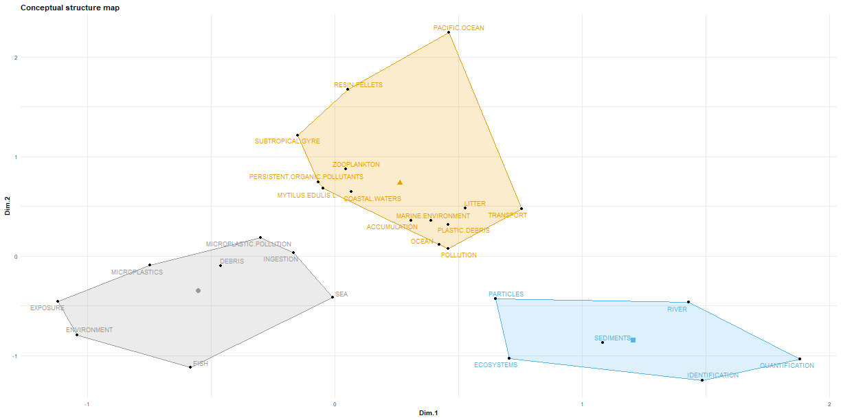
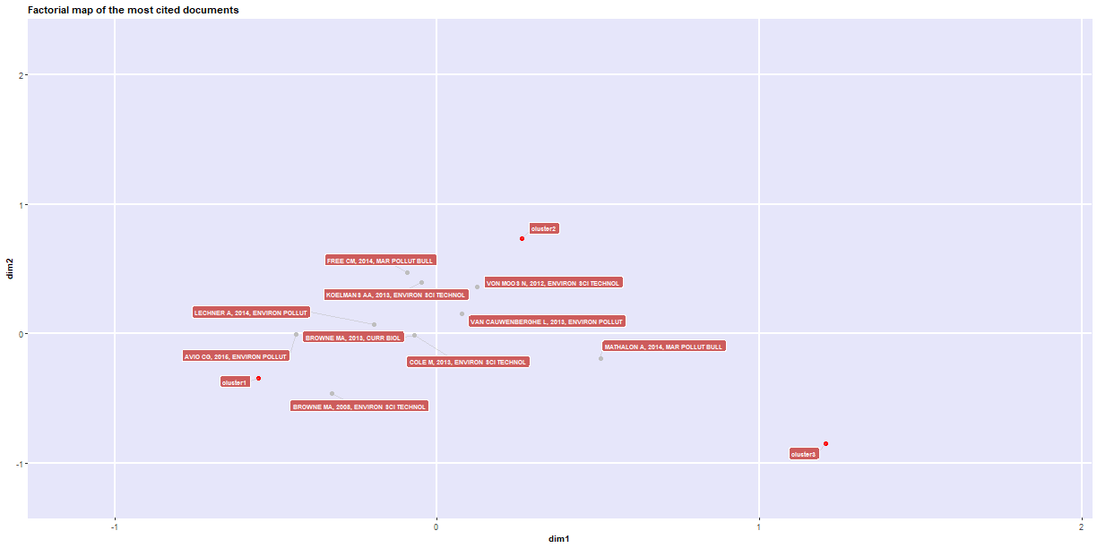
1### We can also look at a conceptual structure plot, where we are basically looking at associations
2### between common terms.
3CS <- conceptualStructure(df.current, field = "ID", method = "MCA", minDegree = 15, k.max = 8, stemming = FALSE,
4    labelsize = 10, documents = 10)

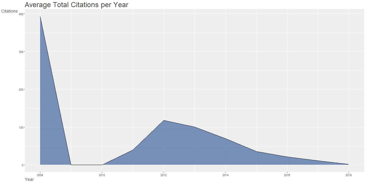
1### We can also look at the direct historical association with a given publication by creating a
2### historical direct citation network.
3histResults <- histNetwork(df.current, min.citations = 20, sep = ".  ")
4
5## Articles analysed   88
6
7net <- histPlot(histResults, n = 10, size = 10, labelsize = 5, size.cex = TRUE, arrowsize = 0.5, color = TRUE)

 1##
 2##  Legend
 3##
 4##                                              Paper                             DOI Year LCS GCS
 5## 2008 - 1      BROWNE MA, 2008, ENVIRON SCI TECHNOL               10.1021/ES800249A 2008  75 393
 6## 2012 - 5     VON MOOS N, 2012, ENVIRON SCI TECHNOL               10.1021/ES302332W 2012  58 216
 7## 2013 - 7                BROWNE MA, 2013, CURR BIOL       10.1016/J.CUB.2013.10.012 2013  41 192
 8## 2013 - 10 VAN CAUWENBERGHE L, 2013, ENVIRON POLLUT    10.1016/J.ENVPOL.2013.08.013 2013  45 198
 9## 2013 - 14        COLE M, 2013, ENVIRON SCI TECHNOL               10.1021/ES400663F 2013  85 325
10## 2014 - 24           FREE CM, 2014, MAR POLLUT BULL 10.1016/J.MARPOLBUL.2014.06.001 2014  46 153
11## 2014 - 26          LECHNER A, 2014, ENVIRON POLLUT    10.1016/J.ENVPOL.2014.02.006 2014  35 124
12## 2015 - 34        COLE M, 2015, ENVIRON SCI TECHNOL         10.1021/ACS.EST.5B04099 2015  41  49
13## 2015 - 43       KLEIN S, 2015, ENVIRON SCI TECHNOL         10.1021/ACS.EST.5B00492 2015  32  93
14## 2015 - 45            AVIO CG, 2015, ENVIRON POLLUT    10.1016/J.ENVPOL.2014.12.021 2015  33 124