Tidyverse Data Wrangling
By Ben Leonard
What is Data Wrangling?
Most of the time datasets will not come "out of the box" ready to use for analysis. Summarizing data and presenting audience friendly tables and figures requires quite a bit of data manipulation. A data wrangling task is performed anytime a dataset is cleaned, tweaked, or adjusted to fit a subsequent analytical step.
Why Use R?
Programs that provide an easy to use graphical user interface (GUI) such as Excel can be used to perform data wrangling tasks. Since it can be faster to manipulate data is Excel why should anyone take extra time to write code in R?
-
Repeatability. A cornerstone of the scientific process is producing a replicable result. If a dataset has to be heavily massaged to produce the desired result these steps must be documented. Otherwise it is easy for errors to creep into the final output. Without transparency it is difficult for reviewers to differentiate between honest mistakes and purposeful data fabrication. It is also difficult to perform any type of quality assurance protocol without proper documentation. By coding all analytical steps in R it is actually easier to leave a trail of evidence showing data wrangling steps than trying to do so in Excel by heavily annotating workbooks.
-
Data Integrity. Excel often does unexpected things to data. For example, Excel will attempt to auto-recognize data types when entering data. If I try to enter the value "1-15" this automatically becomes the date "January 15, 2020". Excel also does not always respect the preservation and display of significant digits. Some formulas don't follow sounds statistical philosophy. Many advanced data maneuvers are absent from or really difficult to perform in Excel.
-
Work Flow. If R is required eventually for statistics, modeling, rmarkdown, shiny, etc. then keeping all steps "in house" just makes sense. Since R and RStudio provide most of the tools a data scientist needs why muddy the waters by switching back and forth with Excel. However, it should be noted that there are many packages that make it easy to integrate the two approaches. For example, readxl is a tidyverse package for reading Excel workbooks. It is also possible to code Excel procedures using Visual Basic for Applications (VBA) code and then programmatically execute this code in R. Many choose a hybrid approach in which Excel is used as a data exploration tool that can be used to figure out which steps need to be taken to accomplish a task in R.
Tidyverse Packages
1# Installing tidyverse packages
2# install.packages("tidyverse")
3
4# Loading tidyverse packages
5# library("tidyverse")
6
7# Tidyverse information
8# ?tidyverse
The tidyverse is an opinionated collection of R packages designed for data science. All packages share an underlying design philosophy, grammar, and data structures.Install the complete tidyverse with:
install.packages("tidyverse")
Loading the tidyverse library is a great way to load many useful packages in one simple step. Several packages included in this distribution are great tools for data wrangling. Notably dplyr, readr, and tidyr are critical assets. The general philosophy is that if a number of steps are needed for a data wrangling task these can be modularized into a stream-lined set into a human readable commands.
Criticism
Some argue that tidyverse syntax is not intuitive and that it should not be taught to students first learning R. Much of the basis for this comes from the avoidance of certain base R staples such as the "$" operator, "[[]]", loops, and the plot command.
https://github.com/matloff/TidyverseSkeptic
Pipe Operator
"%>%"
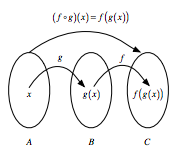
The pipe operator is the crux of all tidyverse data operations. It strings together multiple functions without the need for subsetting. If a number of operations are needed to be performed on a single dataframe this approach simplifies the process. The following image shows the mathematical principle of how the pipe operator works by bridging functions with explicitly subsetting arguments. In this case, steps A %>% B %>% C would represent the tidyverse "pipe syntax" while f(g(x)) is the base R approach.
The examples below show how to perform a few simple tasks in both base R and tidyverse "pipe syntax". Note that for both of these cases the base R syntax may actually be preferred in terms of brevity, but the tidyverse approaches are slightly more readable.
 1## Task #1: Determine the mean of a vector of three doubles.
 2
 3# Create a vector of values
 4a <- c(12.25, 42.50, 75.00)
 5
 6# Base R
 7round(mean(a), digits = 2)
 8
 9## [1] 43.25
10
11# Tidyverse
12a %>%
13  mean() %>%
14  round(digits = 2)
15
16## [1] 43.25
17
18## Task #2: Extract the unique names of all storms in the "storms" dataset and view the first few results.
19
20# Base R
21head(unique(storms$name))
22
23## [1] "Amy"      "Caroline" "Doris"    "Belle"    "Gloria"   "Anita"
24
25# Tidyverse
26storms %>%
27  pull(name) %>%
28  unique() %>%
29  head()
30
31## [1] "Amy"      "Caroline" "Doris"    "Belle"    "Gloria"   "Anita"
Reading Data
read_csv() and write_csv()
While base R does provide analogous functions (read.csv, and write.csv) the versions included in readr are 5 to 10 times faster. This speed, in addition to a loading bar, makes these functions preferred for large files. The dataframes produced are also always tibbles and don't convert columns to factors or use rownames by default. Additionally, read_csv is able to make better determinations about data types and has more sensible defaults.
The example below shows how to read.csv is unable to identify time series data automatically and assigns a column class of "character". However, read_csv correctly reads in the data without having to specify any column data types.
 1## Task #1: Read in a dataset of time series data and determine the default class assignments for each column data type.
 2
 3# Base R
 4sapply(read.csv("weather.csv"), class)
 5
 6##   timestamp       value
 7## "character"   "numeric"
 8
 9# Tidyverse
10read_csv("weather.csv") %>%
11  sapply(class)
12
13## Parsed with column specification:
14## cols(
15##   timestamp = col_datetime(format = ""),
16##   value = col_double()
17## )
18
19## $timestamp
20## [1] "POSIXct" "POSIXt"
21##
22## $value
23## [1] "numeric"
tribble()
Sometimes it is necessary to define a small dataframe in your code rather than reading data from an external source such as a csv file. The tribble() function makes this very easy by allowing row-wise definition of dataframes in tibble format.
Note. A tibble is a type of dataframe specific to the tidyverse. See the following description:
A tibble, or tbl_df, is a modern reimagining of the data.frame, keeping what time has proven to be effective, and throwing out what is not. Tibbles are data.frames that are lazy and surly: they do less (i.e. they don't change variable names or types, and don't do partial matching) and complain more (e.g. when a variable does not exist). This forces you to confront problems earlier, typically leading to cleaner, more expressive code. Tibbles also have an enhanced print() method which makes them easier to use with large datasets containing complex objects.
The example below shows how much more intuitive it is to create data frames using tribble. Row-wise definitions make it simple to enter tabular data and manually update datasets when need be. The use of tribble also guarantees a tibble output which is then going to be fully compatible with all tidyverse functions. A tibble is also achieved without row-wise syntax using tibble() (formerly data_frame()).
 1## Task #2: Manually create a data frame.
 2
 3# Base R
 4class(data.frame("col1" = c(0.251, 2.253),
 5                 "col2" = c(1.231, 5.230)))
 6
 7## [1] "data.frame"
 8
 9# Tidyverse #1
10class(tibble("col1" = c(0.251, 2.253),
11             "col2" = c(1.231, 5.230)))
12
13## [1] "tbl_df"     "tbl"        "data.frame"
14
15# Tidyverse #2
16tribble(
17  ~col1, ~col2,
18  0.251, 1.231,
19  2.253, 5.230,
20  1.295, 3.192, # New Data
21  ) %>%
22  class()
23
24## [1] "tbl_df"     "tbl"        "data.frame"
Manipulating Data
Much of data wrangling comes down to data manipulations performed over and over again. A compact set of functions make this easy in tidyverse without having to nest functions or define a bunch of different variables. While many base R equivalents exist the example below performs a set of commands using only tidyverse syntax.
select() extracts columns and returns a tibble.
arrange() changes the ordering of the rows.
filter() picks cases based on their values.
mutate() adds new variables that are functions of existing variables.
rename() easily changes the name of a column(s)
pull() extracts a single column as a vector.
 1# Task #1: Perform numerous data manipulation operations on a dataset.
 2
 3ToothGrowth %>%
 4  mutate(dose2x = dose*2) %>% # Double the value of dose
 5  select(-dose) %>% # Remove old dose column
 6  arrange(-len) %>% # Sort length from high to low
 7  filter(supp == "OJ") %>% # Filter for only orange juice supplement
 8  rename(length = len) %>% # Rename len to be more explicit
 9  pull(length) %>% # Extract length as a vector
10  head()
11
12## [1] 30.9 29.4 27.3 27.3 26.4 26.4
Summarizing Data
group_by() Most data operations are done on groups defined by variables. group_by() takes an existing tbl and converts it into a grouped tbl where operations are performed "by group". ungroup() removes grouping.
summarize() creates a new data frame. It will have one (or more) rows for each combination of grouping variables; if there are no grouping variables, the output will have a single row summarising all observations in the input. It will contain one column for each grouping variable and one column for each of the summary statistics that you have specified.
summarise() and summarize() are synonyms.
pivot_wider() "widens" data, increasing the number of columns and decreasing the number of rows.
pivot_longer() "lengthens" data, increasing the number of rows and decreasing the number of columns.
Data summarization often requires some difficult maneuvering. Since data summaries may then be used for subsequent analyses and may even be used as a deliverable it is important to have a well documented and clear set of procedures. The following procedures are used to create tabular data summaries much like pivot tables in Excel. However, unlike pivot tables in Excel the steps here are well documented.
 1## Task #1: Summarize the prices of various diamond cuts using a variety of statistical measures and then properly format the results.
 2
 3diamonds %>%
 4  group_by(cut) %>%
 5  summarize(mean = mean(price)) %>%
 6  mutate(mean = dollar(mean))
 7
 8## `summarise()` ungrouping output (override with `.groups` argument)
 9
10## # A tibble: 5 x 2
11##   cut       mean
12##   <ord>     <chr>
13## 1 Fair      $4,358.76
14## 2 Good      $3,928.86
15## 3 Very Good $3,981.76
16## 4 Premium   $4,584.26
17## 5 Ideal     $3,457.54
18
19# Tip: Using _at will apply one or more functions to one or more variables.
20diamonds %>%
21  group_by(cut) %>%
22  summarize_at(vars(price), funs(mean, sd, min, median, max)) %>%
23  mutate_at(vars(-cut), dollar)
24
25## Warning: `funs()` is deprecated as of dplyr 0.8.0.
26## Please use a list of either functions or lambdas:
27##
28##   # Simple named list:
29##   list(mean = mean, median = median)
30##
31##   # Auto named with `tibble::lst()`:
32##   tibble::lst(mean, median)
33##
34##   # Using lambdas
35##   list(~ mean(., trim = .2), ~ median(., na.rm = TRUE))
36## This warning is displayed once every 8 hours.
37## Call `lifecycle::last_warnings()` to see where this warning was generated.
38
39## # A tibble: 5 x 6
40##   cut       mean      sd        min   median    max
41##   <ord>     <chr>     <chr>     <chr> <chr>     <chr>
42## 1 Fair      $4,358.76 $3,560.39 $337  $3,282.00 $18,574
43## 2 Good      $3,928.86 $3,681.59 $327  $3,050.50 $18,788
44## 3 Very Good $3,981.76 $3,935.86 $336  $2,648.00 $18,818
45## 4 Premium   $4,584.26 $4,349.20 $326  $3,185.00 $18,823
46## 5 Ideal     $3,457.54 $3,808.40 $326  $1,810.00 $18,806
47
48## Task #2: a) Create a presence absence table for fish encounters where each station is a different column. b) Then condense the table to get a total fish counts per station.
49
50# a)
51df <- fish_encounters %>%
52  mutate(seen = "X") %>% # Set value to X for seen
53  pivot_wider(names_from = station, values_from = seen) # Move stations to columns
54
55df %>% head()
56
57## # A tibble: 6 x 12
58##   fish  Release I80_1 Lisbon Rstr  Base_TD BCE   BCW   BCE2  BCW2  MAE   MAW
59##   <fct> <chr>   <chr> <chr>  <chr> <chr>   <chr> <chr> <chr> <chr> <chr> <chr>
60## 1 4842  X       X     X      X     X       X     X     X     X     X     X
61## 2 4843  X       X     X      X     X       X     X     X     X     X     X
62## 3 4844  X       X     X      X     X       X     X     X     X     X     X
63## 4 4845  X       X     X      X     X       <NA>  <NA>  <NA>  <NA>  <NA>  <NA>
64## 5 4847  X       X     X      <NA>  <NA>    <NA>  <NA>  <NA>  <NA>  <NA>  <NA>
65## 6 4848  X       X     X      X     <NA>    <NA>  <NA>  <NA>  <NA>  <NA>  <NA>
66
67# b)
68df %>%
69  pivot_longer(-fish, names_to = "station") %>% # Move back to long format
70  group_by(station) %>%
71  filter(!is.na(value)) %>% # Remove NAs
72  summarize(count = n()) # Count number of records
73
74## `summarise()` ungrouping output (override with `.groups` argument)
75
76## # A tibble: 11 x 2
77##    station count
78##    <chr>   <int>
79##  1 Base_TD    11
80##  2 BCE         8
81##  3 BCE2        7
82##  4 BCW         8
83##  5 BCW2        7
84##  6 I80_1      19
85##  7 Lisbon     13
86##  8 MAE         5
87##  9 MAW         5
88## 10 Release    19
89## 11 Rstr       12
Complex Example
While this document follows some pretty simple examples using real-life data can get really complicated quickly. In the last example, I use real data from a study looking at tree transpiration. Data received from Campbell data loggers must be heavily manipulated to calculate "v" or the velocity of sap movement for each timestamp. A function is defined which performs all of the data wrangling steps and allows for the user to change the data sources and censoring protocols. While there is no need to fully understand what is going on with this example it is important to note that each step is documented with in line comments. This tidyverse recipe which is saved as a function can then be added to a custom package and loaded as needed.
 1# Define a function that accomplishes numerous data wrangling steps given several input variables.
 2tdp <- function(
 3  path, # Path to data files
 4  meta, # Name of metadata file
 5  min, # Minimum accepted value
 6  max, # Maximum accepted value
 7  mslope # Minimum accepted slope
 8) {
 9
10  list.files(path = path, # Define subfolder
11                  pattern = "*.dat", # Pattern for file suffix
12                  full.names = TRUE, # Use entire file name
13                  recursive = TRUE) %>% # Create list of dat files
14  map_df(~ read_csv(
15    .x,
16    skip = 4, # Skip first four lines
17    col_names = F, # Don't auto assign column names
18    col_types = cols(), # Don't output
19    locale = locale(tz = "Etc/GMT+8") # Set timezone
20  ) %>% # Read in all dat files
21    select(-c(37:ncol(.))) %>% # Remove extra columns
22    mutate(temp = as.integer(str_extract(.x, "(?<=_)\\d{1}(?=_TableTC.dat)")))) %>% # Extract site number from file name
23  `colnames<-`(c("timestamp", "record", "jday", "jhm", 1:32, "plot_num")) %>% # Manually define column names
24  select(plot_num, everything()) %>% # Move plot_num to be the first column
25  pivot_longer(
26    names_to = "channel",
27    values_to = "dTCa",
28    -(1:5),
29    names_transform = list(channel = as.double)) %>% # Flatten data
30  left_join(read_csv(meta,
31                     col_types = cols())) %>% # Merge tree metadata
32  filter(!is.na(tree_num)) %>% # Remove NAs associated with channels lacking a tree number
33  unite(tree_id,
34        c(plot_num, tree_num, tree_type), # Combine three variables
35        sep = "-", # Use - as delimiter
36        remove = FALSE) %>% # Create tree IDs
37  arrange(plot_num, channel, timestamp) %>%
38  mutate(date = as.Date(timestamp, tz = "Etc/GMT+8"), # Extract date
39         hour = hour(timestamp), # Extract hour of day
40         am = if_else(hour < 12, T, F), # True vs False for morning hours
41         slope = dTCa - lag(dTCa), # Calculate dTCa slope for each timestep
42         flag = ifelse(dTCa < min | dTCa > max | slope > mslope, TRUE, FALSE)) %>% # Flag values that are out of bounds
43  filter(!flag) %>% # Filter and remove values that are out of bounds
44  group_by(plot_num, channel) %>% # Group data by day/site/channel
45  filter(date != min(date)) %>% # Remove first day of data collection
46  group_by(plot_num, channel, date, am) %>% # include date and morning in grouping
47  mutate(dTM = max(dTCa)) %>% # Calculate maximum temperature difference per day/site/channel
48  ungroup() %>%
49  mutate(baseline = if_else(dTCa == dTM & am, dTM, NA_real_), # Force dTM to occur in the morning
50         diff = difftime(timestamp, lag(timestamp), units = "mins"), # Calculate time difference
51         id = if_else(diff != 15 | is.na(diff), 1, 0), # Identify non-contiguous periods of time
52         id = cumsum(id)) %>% # Unique IDs will be produced for contiguous periods of data collection
53  group_by(plot_num, channel, id) %>%
54  mutate(baseline = na.approx(baseline, na.rm = F, rule = 2)) %>% # Interpolate between baselines
55  ungroup() %>%
56  mutate(k = (baseline - dTCa) / dTCa, # Calculate the sap flux index
57         v = 0.0119 * (k ^ 1.231) * 60 * 60, # Calculate sap velocity in cm/hr using Granier formula
58         v = replace_na(v, 0)) %>% # Replace NAs with 0s
59  group_by(tree_id, date, probe_depth) %>%
60  summarize(sum_v = sum(v)) # Select important variables
61}
62
63# Perform data wrangling steps
64tdp(path = "data", meta = "channels.csv", min = 2, max = 20, mslope = 1) %>%
65  head()
66
67## Joining, by = c("plot_num", "channel")
68
69## `summarise()` regrouping output by 'tree_id', 'date' (override with `.groups` argument)
70
71## # A tibble: 6 x 4
72## # Groups:   tree_id, date [2]
73##   tree_id date       probe_depth sum_v
74##   <chr>   <date>           <dbl> <dbl>
75## 1 1-1-DF  2020-07-03          15 155.
76## 2 1-1-DF  2020-07-03          25  79.2
77## 3 1-1-DF  2020-07-03          50 185.
78## 4 1-1-DF  2020-07-03          90  29.6
79## 5 1-1-DF  2020-07-04          15 156.
80## 6 1-1-DF  2020-07-04          25  83.4