Raster analyses in R
By Alli Cramer
Spatial analysis in R
For one of my primary experiences of spatial analysis in R, we used a number of existing data bases to determine the average yearly temperature and precipitation for over 1.3 million lakes. One of my duties in this project was to combine multiple raster layers from a reanalysis of satellite data (From MERRA2, for all you climate nerds) to determine the average values. We then re-sampled the grids to match the spatial resolution of some lake data.
The data is WAY to big to use in this example, so we will first be generating some ncdf files which we will use. Then we will be doing some calculations between the rasters, and mapping them.
If you you like to learn more about spatial calculations in R in general, I recommend this website: https://rspatial.org/spatial/rst/sphere/sphere/index.html
If you would like to learn more specifics about mapping, we have a great mapping tutorial on this blog here: https://cougrstats.netlify.app/post/mapping-in-r/
Libraries you will need
1library(ncdf4)
2library(raster)
3library(rasterVis)
4library(maptools)
5library(maps)
6library(gridExtra)
Our For Fun data
This section is long, just scroll past it if you want to get to the "how" and not the "fake data" bit.
Our for fun data are NetCDF files. NetCDFs are very compact, easily machine read file formats that are frequently used to store large data sets. Most of the climate, oceanographic, or population spatial data from governmental sources are in this format, so it is useful to be exposed to it. They are, however, a bit difficult to read for humans. One way to easily view a netCDF file, and all of the subsequent layers and metadata, is with Panoply, a free viewer from NOAA.
We will not be discussing the format of netCDF files, we will just be making two small ones to play with. A good discussion of netCDFs in R can be found at this University of Oregon site.
 1library(ncdf4)
 2#code modified from http://geog.uoregon.edu/GeogR/topics/netcdf-to-raster.html
 3
 4# create a small netCDF file, save, and read back in using raster and rasterVis
 5# generate lons and lats
 6nlon <- 24; nlat <- 9
 7dlon <- 360.0/nlon; dlat <- 180.0/nlat
 8lon <- seq(-180.0+(dlon/2),+180.0-(dlon/2),by=dlon)
 9lat <- seq(-90.0+(dlat/2),+90.0-(dlat/2),by=dlat)
10
11# generate the first temperature data
12set.seed(10) # for reproducibility
13tmp1 <- rnorm(nlon*nlat)
14tmat <- array(tmp1, dim = c(nlon, nlat))
15
16# define dimensions
17londim <- ncdim_def("lon", "degrees_east", as.double(lon))
18latdim <- ncdim_def("lat", "degrees_north", as.double(lat))
19
20# define variables
21varname="tmp"
22units="z-scores"
23dlname <- "test variable -- original"
24fillvalue <- 1e20
25tmp.def <- ncvar_def(varname, units,
26                    list(londim, latdim),
27                    fillvalue,  dlname,
28                    prec = "single")
29
30# create a netCDF file
31ncfname <- "test-netCDF-file_tmp1.nc"
32ncout <- nc_create(ncfname, list(tmp.def), force_v4 = TRUE)
33
34# put the array
35ncvar_put(ncout, tmp.def, tmat)
36
37# put additional attributes into dimension and data variables
38ncatt_put(ncout, "lon", "axis", "X")
39ncatt_put(ncout, "lat", "axis", "Y")
40
41# add global attributes
42title <- "small example netCDF file"
43ncatt_put(ncout, 0, "title", title)
44
45# close the file, writing data to disk
46nc_close(ncout)
47
48# generate the second temperature data
49set.seed(12) # for reproducibility
50tmp2 <- rnorm(nlon*nlat)
51tmat <- array(tmp2, dim = c(nlon, nlat))
52
53# define dimensions
54londim <- ncdim_def("lon", "degrees_east", as.double(lon))
55latdim <- ncdim_def("lat", "degrees_north", as.double(lat))
56
57# define variables
58varname="tmp"
59units="z-scores"
60dlname <- "test variable -- original"
61fillvalue <- 1e20
62tmp.def <- ncvar_def(varname, units,
63                    list(londim, latdim),
64                    fillvalue,  dlname,
65                    prec = "single")
66
67# create a netCDF file
68ncfname <- "test-netCDF-file_tmp2.nc"
69ncout <- nc_create(ncfname, list(tmp.def), force_v4 = TRUE)
70
71# put the array
72ncvar_put(ncout, tmp.def, tmat)
73
74# put additional attributes into dimension and data variables
75ncatt_put(ncout, "lon", "axis", "X")
76ncatt_put(ncout, "lat", "axis", "Y")
77
78# add global attributes
79title <- "small example netCDF file"
80ncatt_put(ncout, 0, "title", title)
81
82# close the file, writing data to disk
83nc_close(ncout)
Rasters
First, what is a raster?
A raster is a type of data structure which exists in an array. Rasters are analogous to digital photos - every grid cell, or pixel, has a value. In a photo that value is a color. For rasters, that value can be a variety of things - temperature, population, etc.
Rasters are useful when doing spatial analyses because programs that understand rasters can perform calculations on the same grid cell by default - aka when using a raster programs "know" that you want calculations performed on a cell by cell basis. Otherwise, we have to write loops etc. to explicitly tell the computer that "hey, I want cell b5 to be subtracted from b5, and cell b6 to be subtracted from b6,..." and so on. If you do NOT want this type of cell to cell math, then a raster might not be for you. But if you DO, they can be a life saver.
Raster calculations
One of the primary uses for rasters is to compare one set of spatial data to another. For example, we can compare temperature vs precipitation, or the elevation of an area vs it's slope. You may have used GIS to do this before, and the benefit of the GIS framework is that it double checks many of your steps. It is, however, slow.
When using rasters in R make sure to double check your
- projection
- dimensions
- expected values
Before doing any calculations
Our for fun data
Our for fun data is ncdf data. Ncdf files are different file formats from raster, but they can be READ as rasters by the raster package in R. Lets explore our ncdf and one of our raster files.
 1#reading in the raster
 2library(raster)
 3library(rasterVis)
 4library(maptools)
 5library(maps)
 6
 7T1.nc <- nc_open("test-netCDF-file_tmp1.nc")
 8T1.nc
 9
10## File test-netCDF-file_tmp1.nc (NC_FORMAT_NETCDF4):
11##
12##      1 variables (excluding dimension variables):
13##         float tmp[lon,lat]   (Contiguous storage)
14##             units: z-scores
15##             _FillValue: 1.00000002004088e+20
16##             long_name: test variable -- original
17##
18##      2 dimensions:
19##         lon  Size:24
20##             units: degrees_east
21##             long_name: lon
22##             axis: X
23##         lat  Size:9
24##             units: degrees_north
25##             long_name: lat
26##             axis: Y
27##
28##     1 global attributes:
29##         title: small example netCDF file
30
31nc_close(T1.nc)
32
33T1 <- raster("test-netCDF-file_tmp1.nc")
34T2<- raster("test-netCDF-file_tmp2.nc")  # we aren't going to look at this, but lets bring it in to save for later
35T1
36
37## class       : RasterLayer
38## dimensions  : 9, 24, 216  (nrow, ncol, ncell)
39## resolution  : 15, 20  (x, y)
40## extent      : -180, 180, -90, 90  (xmin, xmax, ymin, ymax)
41## coord. ref. : +proj=longlat +datum=WGS84 +ellps=WGS84 +towgs84=0,0,0
42## data source : C:\Users\allison.cramer\OneDrive\Teaching\R Working Group\WriteUps\test-netCDF-file_tmp1.nc
43## names       : test.variable....original
44## zvar        : tmp
45
46print(T1)
47
48## File C:\Users\allison.cramer\OneDrive\Teaching\R Working Group\WriteUps\test-netCDF-file_tmp1.nc (NC_FORMAT_NETCDF4):
49##
50##      1 variables (excluding dimension variables):
51##         float tmp[lon,lat]   (Contiguous storage)
52##             units: z-scores
53##             _FillValue: 1.00000002004088e+20
54##             long_name: test variable -- original
55##
56##      2 dimensions:
57##         lon  Size:24
58##             units: degrees_east
59##             long_name: lon
60##             axis: X
61##         lat  Size:9
62##             units: degrees_north
63##             long_name: lat
64##             axis: Y
65##
66##     1 global attributes:
67##         title: small example netCDF file
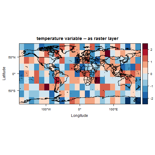
As you can see, the data is stored differently between the ncdf and the raster. However, by comparing the two files you can see that the raster package, with the raster() function, opened the ncdf correctly and interpreted it right. We can now move on to mapping our raster file.
1# map the data
2world.outlines <- map("world", plot=FALSE)
3world.outlines.sp <- map2SpatialLines(world.outlines, proj4string = CRS("+proj=longlat"))
4
5mapTheme <- rasterTheme(region = rev(brewer.pal(10, "RdBu")))
6cutpts <- c(-2.5, -2.0, -1.5, -1, -0.5, 0, 0.5, 1.0, 1.5, 2.0, 2.5)
7plt <- levelplot(T1, margin = F, at=cutpts, cuts=11, pretty=TRUE, par.settings = mapTheme,
8  main="temperature variable -- as raster layer")
9plt + layer(sp.lines(world.outlines.sp, col = "black", lwd = 0.5))
Raster Brick and Raster Stack
Often, rasters have multiple layers, or "bands". To open a multi-band raster we use the brick() function from the raster package.
But what if we want to open multiple rasters and then do some calculations? Say ... average temperature?
For this, we use the stack() function. A raster stack is less efficient than a brick, so if doing large computations it can be efficient to use stack to then create bricks, and then do calculations. Lets try getting average temperature from our two ncdf files.
 1#look for the .nc files in the directory
 2ncs <- list.files(getwd(), pattern = "*.nc$")
 3
 4#create a raster stack from the files
 5stacked <- raster::stack(ncs)
 6
 7#lets do some math!
 8
 9#calculate mean temperature for every grid cell in the raster, between the two layers
10Tmean <- mean(stacked)
11
12#Lets check it
13Tmean
14
15## class       : RasterLayer
16## dimensions  : 9, 24, 216  (nrow, ncol, ncell)
17## resolution  : 15, 20  (x, y)
18## extent      : -180, 180, -90, 90  (xmin, xmax, ymin, ymax)
19## coord. ref. : +proj=longlat +datum=WGS84 +ellps=WGS84 +towgs84=0,0,0
20## data source : in memory
21## names       : layer
22## values      : -1.427061, 2.079051  (min, max)
23
24#save this new calculated raster as a GeoTiff
25writeRaster(Tmean, filename = "test-GTiff-file_TmpMean.tif", format="GTiff", overwrite = TRUE)
Comparing the Data
 1T1
 2
 3## class       : RasterLayer
 4## dimensions  : 9, 24, 216  (nrow, ncol, ncell)
 5## resolution  : 15, 20  (x, y)
 6## extent      : -180, 180, -90, 90  (xmin, xmax, ymin, ymax)
 7## coord. ref. : +proj=longlat +datum=WGS84 +ellps=WGS84 +towgs84=0,0,0
 8## data source : C:\Users\allison.cramer\OneDrive\Teaching\R Working Group\WriteUps\test-netCDF-file_tmp1.nc
 9## names       : test.variable....original
10## zvar        : tmp
11
12T2
13
14## class       : RasterLayer
15## dimensions  : 9, 24, 216  (nrow, ncol, ncell)
16## resolution  : 15, 20  (x, y)
17## extent      : -180, 180, -90, 90  (xmin, xmax, ymin, ymax)
18## coord. ref. : +proj=longlat +datum=WGS84 +ellps=WGS84 +towgs84=0,0,0
19## data source : C:\Users\allison.cramer\OneDrive\Teaching\R Working Group\WriteUps\test-netCDF-file_tmp2.nc
20## names       : test.variable....original
21## zvar        : tmp
22
23Tmean
24
25## class       : RasterLayer
26## dimensions  : 9, 24, 216  (nrow, ncol, ncell)
27## resolution  : 15, 20  (x, y)
28## extent      : -180, 180, -90, 90  (xmin, xmax, ymin, ymax)
29## coord. ref. : +proj=longlat +datum=WGS84 +ellps=WGS84 +towgs84=0,0,0
30## data source : in memory
31## names       : layer
32## values      : -1.427061, 2.079051  (min, max)
33
34# Setting up the maps
35world.outlines <- map("world", plot=FALSE)
36world.outlines.sp <- map2SpatialLines(world.outlines, proj4string = CRS("+proj=longlat"))
37
38mapTheme <- rasterTheme(region = rev(brewer.pal(10, "RdBu")))
39cutpts <- c(-2.5, -2.0, -1.5, -1, -0.5, 0, 0.5, 1.0, 1.5, 2.0, 2.5)
40
41#T1 plot
42plt_1 <- levelplot(T1, margin = F, at=cutpts, cuts=11, pretty=TRUE, par.settings = mapTheme,
43  main="T1 -- as raster layer")
44
45#T2 plot
46plt_2 <- levelplot(T2, margin = F, at=cutpts, cuts=11, pretty=TRUE, par.settings = mapTheme,
47  main="T2 -- as raster layer")
48
49#Tmean plot
50plt_m <- levelplot(Tmean, margin = F, at=cutpts, cuts=11, pretty=TRUE, par.settings = mapTheme,
51  main="Tmean -- as raster layer")
52
53#Actual plots
54library(gridExtra) #to put our plots all next to each other all fancy
55
56p1 <- plt_1 + layer(sp.lines(world.outlines.sp, col = "black", lwd = 0.5))
57p2 <- plt_2 + layer(sp.lines(world.outlines.sp, col = "black", lwd = 0.5))
58pm <- plt_m + layer(sp.lines(world.outlines.sp, col = "black", lwd = 0.5))
59
60grid.arrange(
61  arrangeGrob(p1, p2, ncol = 2),  #put plots p1 & p2 next to each other on the same row, in 2 columns (ncol=columns)
62  pm, nrow = 2, #put pm on the next row, out of two rows (nrow=rows)
63  heights = c(1,1.5)) #make the second row larger (here it is 1.5)
